When Leibniz came to Paris in 1672, his mathematical knowledge was rather scant. It was through his acquaintance with Ch. Huygens, one of the leading mathematicians of his time in Europe, that Leibniz’s interest in Mathematics sparked. One of the problems that Huygens proposed was that of finding the sum of the series of the reciprocals of triangular numbers
Realizing that the terms in the series were the successive differences between the terms of the sequence
Leibniz concluded that the th partial sums of the former sequence were equal to the difference between the -th term and the first term of the latter, that is (this device is what we call telescoping). He developed this idea, considering sequences of differences of differences (second differences), third differences, etc. Thus, one can move “up” and “down” along the sequence of successive differences, establishing relations between the sums of differences and the net change of the generating sequence.
Perhaps the simplest example is that of arithmetic sequences . In this case, the sequence of differences is constant, . The sum of the first differences is just hence or . Arithmetic sequences are just linear functions of .
Now, what if the differences of the original sequence form an arithmetic sequence and the second differences are constant?
Suppose the original sequence is , the sequence of first differences is where and the sequence of second differences is with , a constant. We know that is an arithmetic sequence with difference , hence . Hence
,
Adding all the relations above and taking into account the cancelations on the left hand side (telescopic effect) we obtain
or
Observe the following: a) is given by a second degree polynomial; b) the free term is the first element of the sequence , the coefficient of the linear term is , the first “first difference”, and the coefficient of the quadratic part is , which is the constant value of the second difference. At this point it should be clear that we can extend this procedure to the case when the third differences or, more generally, the differences of a certain order are constant. Unsurprisingly, we get polynomials of degree equal to the order of the constant difference, where the coefficients only depend on the first values of consecutive differences. This is what we could call a “discrete” (and finite) Taylor series.
Leibniz was, above all, a philosopher. He realized that he could extend this methods to functions of a continuous variable. But then he would have to replace the differences by infinitesimal differences between to “successive” values of the variable. He had been thinking about the concept of infinitesimal for years, particularly through correspondence with Hobbes and his concept of “conatus“. All the pieces came together in his mind, leading to the creation of infinitesimal Calculus within a few years. Simultaneously, he introduced the notation for successive “differentials”: etc. and integrals (“summa omnia”) for the above processes of moving “down” and “up”, but this time applied to functions of a continuous variable. The passage becomes . We deal with the continuous case in the next post.
Nowadays, we conceive Calculus as the study of functions. The concept of function, originated with Leibniz, was not defined in its full generality until the mid 1800s by Dirichlet. But in the early development of Calculus, the main objects of Calculus were variable quantities, notably those that varied together. For example, Euler considered quantities that vanish or increase infinitely in his famous Introductio in analysin infinitorum, from 1748. Such dynamic view of quantities is one of the features that have been lost or, at least obscured by the modern approach, based on limits. The definition is a bit too “algebraic” and static: the dynamics is encoded in the conditional “ such that..” Euler’s “quantities”, in contrast, had a variable nature.
A quantity that we can consider as becoming ever smaller is called an infinitesimal. A possible mental image is that of a segment which increasingly diminishes until it becomes a single point, or an angle whose sides become closer and closer until they coincide. In modern terminology, an infinitesimal is a variable whose limit is zero. If a variable quantity is approaching some (finite) value , the difference is an infinitesimal.
Calculus is concerned with simultaneous variations of related quantities. Thus for example we can consider the variation of the area of a square of side when its side is increased/decreased by an infinitesimal amount. Such infinitesimal amount was denoted by Leibniz, the Bernoullis, Euler, etc. and even today by physicist, engineers, etc, by , and is called a differential. A simple computation gives the new area
The corresponding change of area is , which is another infinitesimal. In modern terminology, we say that the area is a continuous function of the side: if the side is infinitesimally increased/decreased, the area changes infinitesimally. In most applications to Physics and Engineering, we deal with continuous functions.
A central idea to Calculus is that infinitesimals can be classified according to the relative speed with which they approach zero. It does not make sense to talk about the speed of one infinitesimal, but it does make sense to talk about whether two related infinitesimals (as the ones considered above) approach zero at a comparable speed. Thus if is an infinitesimal quantity, the related infinitesimal approaches zero much faster, since their ratio is itself infinitesimal. We all know that if we look at a sequence of values like , their squares form a sequence that approaches zero much faster; . The infinitesimal approaches zero even faster since the ratio is again an infinitesimal.
These considerations lead to the concept of order of infinitesimals. Namely, given two related infinitesimals and , we say that is of a higher order (than ) if their ratio is infinitesimal. A nice notation introduced by E. Landau and widely used in Computer Science is that of “little o”. Using the “little o” notation, we write
In modern terminology, we would say: given two functions and with , we say that if . This is nice and clean, but one has the impression that the dynamics is somehow lost.
In many instances, two related infinitesimals are “comparable”. Back to the previous example of the area as a function of the side, the quotient
is not an infinitesimal, but takes values closer and closer to instead. In such cases we use the “big O” notation. For generic related infinitesimals and as above, we would write
Thus, .
In the particular case when the ratio approaches , we say that the infinitesimals are equivalent. That means, of course, the given infinitesimals take very close values as they vanish. Equivalency is denotes by the symbol ““
It seems to me that the qualitative aspect of the concept of order is not sufficiently stressed. Even the suggestive “little o” notation is not used in many of the standard current undergraduate Calculus textbooks, including J. Stewart’s, Edwards & Penney, Larson & Edwards, and many others. I think this is very unfortunate, and is part of a general tendency to avoid “qualitative” and “synthetic” reasoning, favoring quantitave and procedural aspects instead.
An interesting infinitesimal is , where is an infinitesimal angle. In the figure below, the radius is chosen to be one for simplicity. The following inequalities are obvious.
or, equivalently,
which, after dividing by throughout, becomes
,
the latter equality being a consequence of similarity of triangles and .
Clearly, as approaches zero, approaches one. As a consequence. The ratio , being trapped between two quantities approaching one, also approaches one. Using the above terminology, and are equivalent infinitesimals, . In the language of limits
.
A vivid example of infinitesimals of different orders is given by the different segments, areas, etc. determined on a circle by an infinitesimal angle .
When the angle is infinitesimal, the following quantities (functions of the angle): and the area of the yellow circular segment are related infinitesimals. is just a linear function of so which is a non-zero constant. Therefore . Next, we see that which, according to the previous example, is equivalent to . Therefore, . As for , we have
.
Since , and .
Finally, the area of the segment is
On the right hand side, we have the difference between two equivalent infinitesimals. What is the order of that? I will leave the question open at this point, and will come back to it in my next post, where we will deal with successive differences and differentials.


 definition is a bit too “algebraic” and static: the dynamics is encoded in the conditional “
 such that..” Euler’s “quantities”, in contrast, had a variable nature.
 is approaching some (finite) value
  , the difference
  is an infinitesimal.
  when its side is increased/decreased by an infinitesimal amount. Such infinitesimal amount was denoted by Leibniz, the Bernoullis, Euler, etc. and even today by physicist, engineers, etc, by
  , and is called a differential. A simple computation gives the new area
 , which is another infinitesimal. In modern terminology, we say that the area is a continuous function of the side: if the side is infinitesimally increased/decreased, the area changes infinitesimally. In most applications to Physics and Engineering, we deal with continuous functions.
  is an infinitesimal quantity, the related infinitesimal
  approaches zero much faster, since their ratio
  is itself infinitesimal. We all know that if we look at a sequence of values like
  , their squares form a sequence that approaches zero much faster;
  . The infinitesimal
  approaches zero even faster since the ratio
  is again an infinitesimal.
  is infinitesimal. A nice notation introduced by E. Landau and widely used in Computer Science is that of “little o”. Using the “little o” notation, we write
 and
and  with
with  , we say that
  if
if  . This is nice and clean, but one has the impression that the dynamics is somehow lost.
 instead. In such cases we use the “big O” notation. For generic related infinitesimals
 .
. , we say that the infinitesimals are equivalent. That means, of course, the given infinitesimals take very close values as they vanish. Equivalency is denotes by the symbol “
 “
“ , where
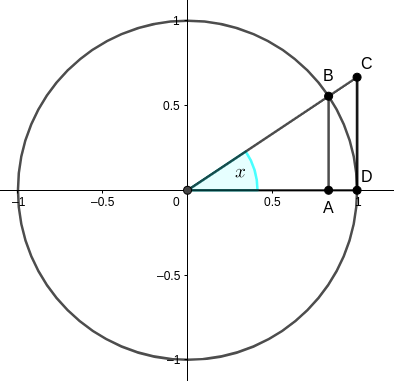


 throughout, becomes
 ,
, and
and  .
. approaches one. As a consequence. The ratio
  , being trapped between two quantities approaching one, also approaches one. Using the above terminology,
  . In the language of limits
 .
. .
.
 and the area of the yellow circular segment are related infinitesimals.
  is just a linear function of
  which is a non-zero constant. Therefore
  . Next, we see that
  which, according to the previous example, is equivalent to
  . Therefore,
  . As for
  .
. ,
,  and
and  .
.
