In simple instances, tangency can be easily characterized. For example, a straight line is tangent to a circle precisely when they share a unique point. More generally, a curve which is the smooth boundary of a convex set has a unique tangent at each point, which can be characterized as the supporting line of the convex set.
But in more general cases such description is inadequate. For example, how do we characterize the tangent to the graph of a polynomial like 


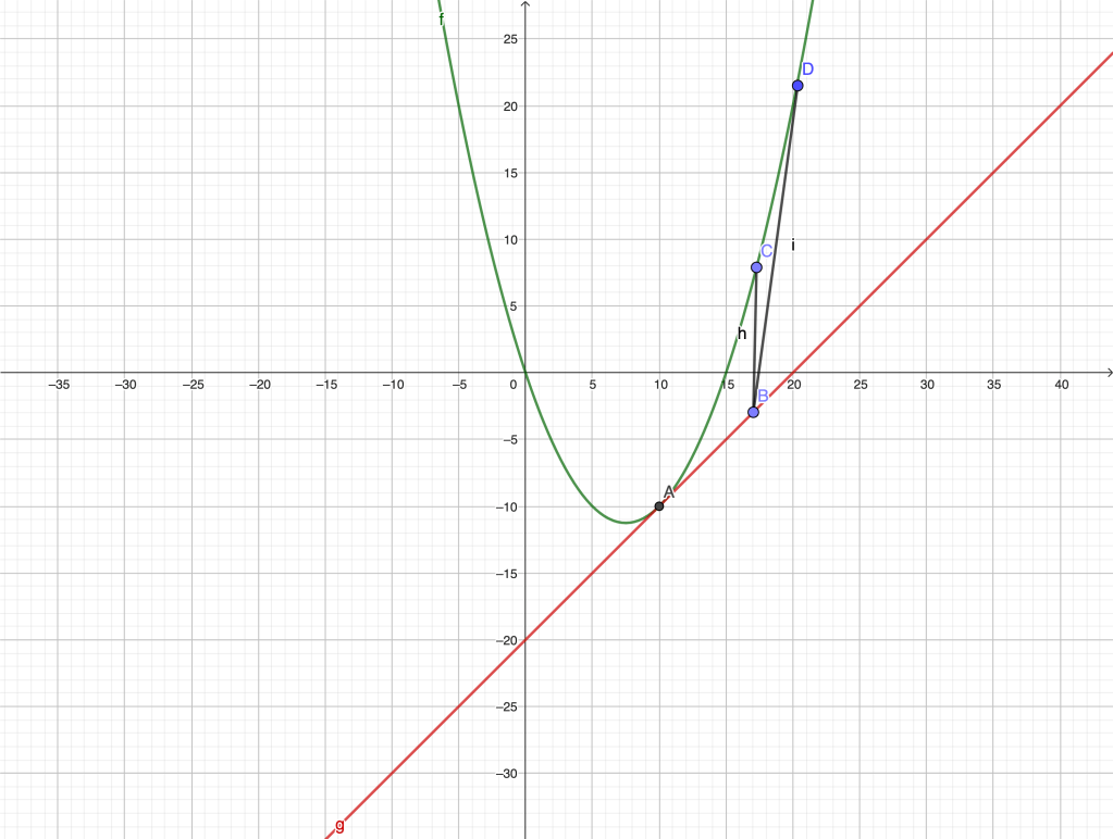
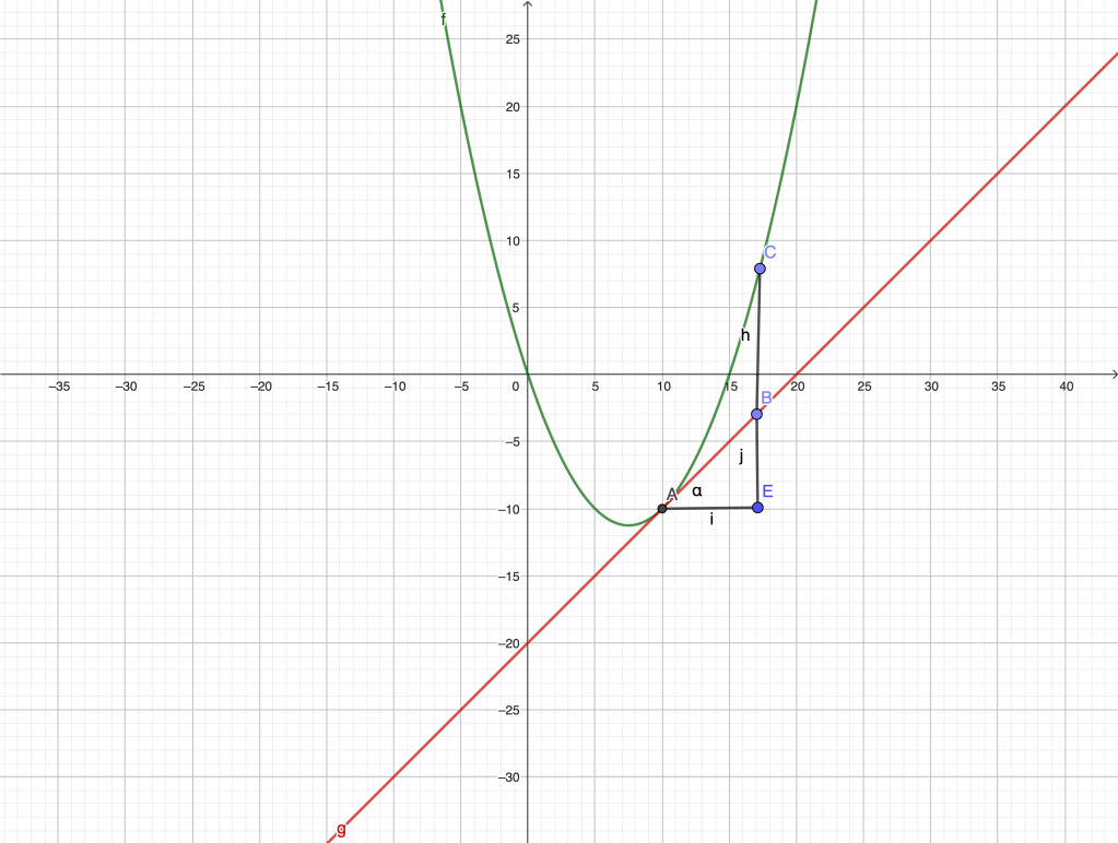
Finding tangents, along with finding areas, is one of the geometric problems that gave impetus to the use of infinitesimals and the eventual creation of Calculus. Predecessors of Newton and Leibniz, notably Fermat and Descartes, devised methods for finding tangents. For example, according to Fermat’s method, to find the tangent to the graph below at 


or, calling 

This, in turn, can be written as

Expanding and simplifying the left hand side and setting 


These ideas were further refined by Roverbal, Wallis, Barrow, Newton and Leibniz. The latter defined the tangent as the line through a pair of infinitely close points on the curve.
The modern analytic characterization is the following: the tangent line at a point of a curve has to be such that, as we move along the tangent towards the point of intersection with the curve, the distance to the graph in any “transversal” direction decreases to zero faster than the distance “along” the tangent to the point of intersection. That is, the curve is “transversally” closer to the tangent near the given point. In a sense, the neglect of the transversal separation between the triangles 

The line 


when 


Notice that, for a non-tangent, transversal line through 
It follows from our definition that the tangent is unique (if there is one). It is also worth noting that the concept of tangency belongs to Euclidean, as well as to affine geometries: tangency does not break down under rigid motions, translations and more general affine transformations (shear, dilations, etc.)
It is natural to quantify the “amount” of tangency by the order of the infinitesimal 


So, in particular, the order of tangency is zero if the line is transversal to the curve, it is one if
Tangents and differentiability
The existence of the tangent to the curve 


when 
If we assume that the straight line 
![|BC|=y(x)-[y_0+m(x-x_0)]=o(|x-x_0|)](https://s0.wp.com/latex.php?latex=%7CBC%7C%3Dy%28x%29-%5By_0%2Bm%28x-x_0%29%5D%3Do%28%7Cx-x_0%7C%29&bg=ffffff&fg=444444&s=0&c=20201002)
or

But this is precisely our definition of differentiable function at 


If the order of tangency is 

it follows from the definition that 

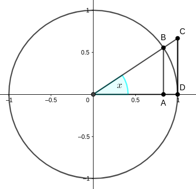
As an example, let’s examine the order of tangency between a circle and its tangent at some point. For simplicity, consider the circle

with unit radius, center 

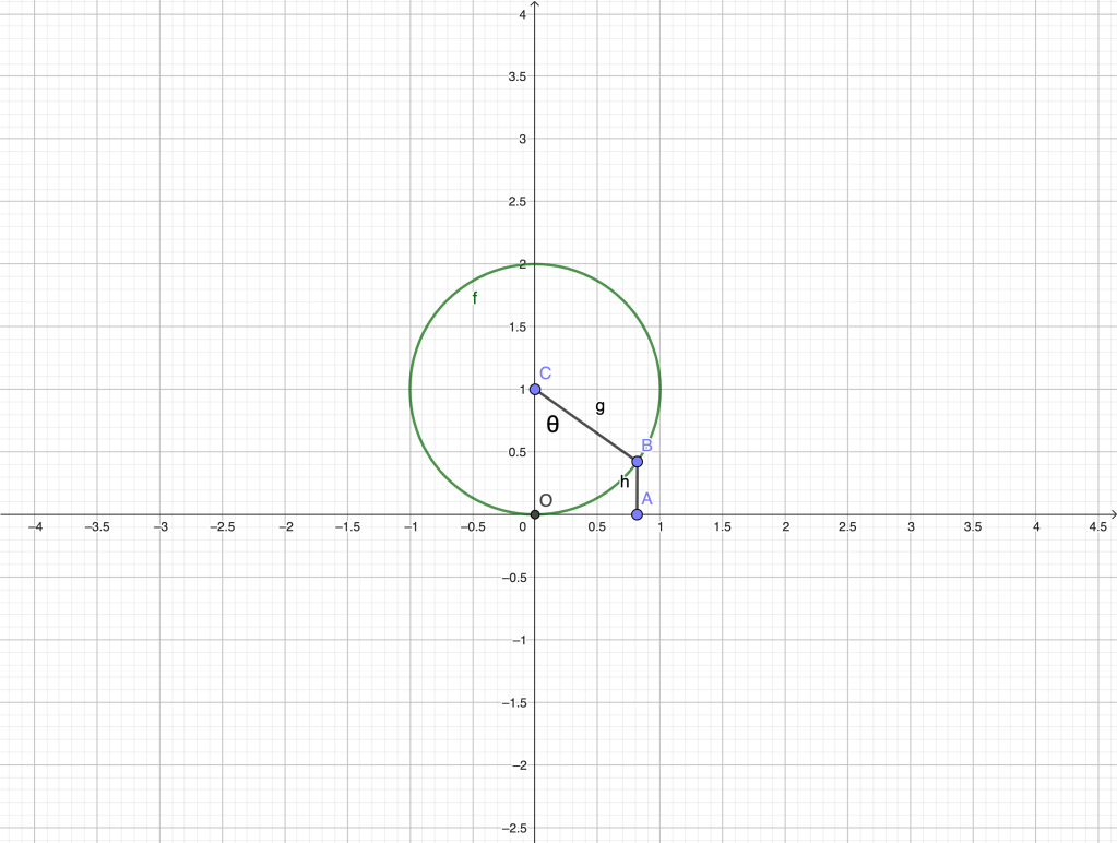
We have 


as 


as 

The value of the limit 


The usual (linear) angle between a circle and its tangent at one point is zero. But our previous analysis allows to quantify the separation between the circle and the tangent using an infinitesimal quadratic scale. Observe that when 
Angles like the above, whose usual measure is zero but their extent can be quantified as before, have been known since antiquity.
Horn angles
A horn angle is the angle formed between a circle and its tangent or, more generally, between two tangent circles at their point of tangency. Given two circles internally tangent, it is natural to define the measure of the horn angle between them as the difference of the angles they form with their common tangent. If they are externally tangent, we take the sum instead, as in the figure below.
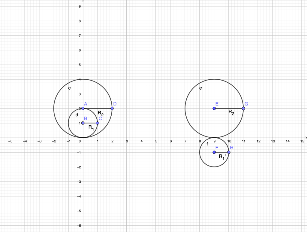
Thus, 


Horn angles are mentioned by Euclid in Book III (Prop. 16) of the “Elements”, and were known to Archimedes and Eudoxus. Euclid states that a horn angle is “smaller than any acute angle”. That property made horn angles problematic to Ancient Greek mathematicians, since they always assumed that any two “homogeneous” magnitudes (lengths, angles, areas, ..) were comparable, in the sense that anthyphairesis (as we would say today, the Euclidean algorithm) could be applied to them. At the end of the process, commensurable magnitudes could be assigned numbers with respect to some unit. Incommensurable magnitudes could not, but the situation could be handled by means of Eudoxus’ theory of proportions, a predecessor of Dedekind’s theory of real numbers. But the notion of a non-zero angle smaller than any acute angle was out of grasp. In modern terminology, we would say that the Archimedean property of segments, angles, areas was a basic assumption in Greek geometry.
We have been able to define a measure for horn angles using the concept of order of infinitesimals. However, to restore the Greeks’ assumption on the possibility to compare (albeit “in the limit”) any pair of angles, actual infinitesimal angles of different orders need to be included in the picture. This is the content of non-Archimedean Geometry, based on the construction of non-Archimedean fields (surreal, hyperreal numbers) in Nonstandard Analysis. The development of these ideas is a very interesting chapter of Analysis, well deserving a separate post, or even a separate thread.
 of its side equals
 , corresponding to a change
  :
:
 .
. is given by the linear (in
  of a variable
  ,
, , we say that
  is differentiable at
  . The coefficient
  is what we call the derivative of
  . Finding the derivative from the knowledge of
  involves, in the general case, considering
  infinitesimal (see below). For polynomials, however, it only requires algebraic manipulations.
 at a generic
 ![\Delta y=(x+dx)^3+2(x+dx)^2+(x+dx)-1-[ x^3+2x^2+x-1]=](https://s0.wp.com/latex.php?latex=%5CDelta+y%3D%28x%2Bdx%29%5E3%2B2%28x%2Bdx%29%5E2%2B%28x%2Bdx%29-1-%5B+x%5E3%2B2x%5E2%2Bx-1%5D%3D&bg=ffffff&fg=444444&s=0&c=20201002)


 , the total variations of
  is a polynomial of degree
  , and we look at the change of
  , we will have
 depending on the base point
  , we just expand the powers
  according to Newton’s binomial theorem. We can think of the coefficients as rates of different orders, multiplying the corresponding powers of
  : the rates, which depend only on the base point, and the different powers of the variation of the independent variable
  or
or  a similar expansion holds. The key difference is that the expansion may contain infinitely many terms. Thus, the concept of a power series serves as a bridge between algebraic and transcendental relations. The idea that (at least smooth) functional relations are either polynomials or “infinite degree polynomials” (power series) dominated Analysis over a long period of time. Newton himself considered the binomial series and the use of series in general to solve differential equations his main mathematical achievement. They also allowed to define many non-elementary functions and to develop Complex Analysis. Series were informally used by Euler, Lagrange, Laplace and many others, in some cases producing paradoxical results. Questions related to convergence were not posed until the middle of the XIX century by Gauss, Abel, Cauchy, etc. It is said that when Laplace heard about Cauchy’s convergence criteria, he rushed home to check the series he used in his monumental “Celestial Mechanics”. Luckily for him and for the stability of the Solar System, all of them were convergent in the range of parameters he considered.
 etc. simply as
  etc. As
  . This is how the (first) derivative is usually defined,


 is typically quadratic,
  or of a higher order,
  if
if  . It is natural that the quadratic correction
  is related to the variation of
  over the interval
  . Thus, we introduce the second differential of

 ,
, ,
, is the derivative of the first derivative
  related to
  and, at that point, use


![= \displaystyle{\frac{[A(x+dx/2)-A(x)]dx/2+[B(x+dx/2)+B(x)](dx/2)^2+\dots}{(dx)^2}}](https://s0.wp.com/latex.php?latex=%3D+%5Cdisplaystyle%7B%5Cfrac%7B%5BA%28x%2Bdx%2F2%29-A%28x%29%5Ddx%2F2%2B%5BB%28x%2Bdx%2F2%29%2BB%28x%29%5D%28dx%2F2%29%5E2%2B%5Cdots%7D%7B%28dx%29%5E2%7D%7D&bg=ffffff&fg=444444&s=0&c=20201002) ,
, . In the limit
  we obtain
 ,
, .
. ![[x,x+dx]](https://s0.wp.com/latex.php?latex=%5Bx%2Cx%2Bdx%5D&bg=ffffff&fg=444444&s=0&c=20201002) into three equal pieces, since we want to account for the variation of the second differential, which depends on three points. Precisely, we introduce the third differential of
into three equal pieces, since we want to account for the variation of the second differential, which depends on three points. Precisely, we introduce the third differential of  .
. ,
, is called the third derivative of
 . In general, we define the
 . The total variation of a polynomial of degree
  .
.  can be dealt with the same way, leading to their power (Taylor) expansions:
 can be expressed in the form
  , then
  , etc are uniquely determined in terms of the derivatives. The question as to whether such a representation is at all available, even for infinitely differentiable functions, leads to the concept of analytic function, to be considered in a future post.

 -th term and the first term of the latter, that is
  (this device is what we call telescoping). He developed this idea, considering sequences of differences of differences (second differences), third differences, etc. Thus, one can move “up” and “down” along the sequence of successive differences, establishing relations between the sums of differences and the net change of the generating sequence.
  . In this case, the sequence of differences is constant,
  . The sum of the first
  hence
hence  or
or  . Arithmetic sequences are just linear functions of
  , the sequence of first differences is
  where
where  and the sequence of second differences is
  with
with  , a constant. We know that
  is an arithmetic sequence with difference
  , hence
  . Hence
 ,
,


 is given by a second degree polynomial; b) the free term is the first element of the sequence
  , the coefficient of the linear term is
  , the first “first difference”, and the coefficient of the quadratic part is
  are constant. Unsurprisingly, we get polynomials of degree equal to the order of the constant difference, where the coefficients only depend on the first values of consecutive differences. This is what we could call a “discrete” (and finite) Taylor series.
  etc. and integrals (“summa omnia”)
  for the above processes of moving “down” and “up”, but this time applied to functions of a continuous variable. The passage
  becomes
  . We deal with the continuous case in the next post.
 definition is a bit too “algebraic” and static: the dynamics is encoded in the conditional “
 such that..” Euler’s “quantities”, in contrast, had a variable nature.
 , the difference
  is an infinitesimal.
 , which is another infinitesimal. In modern terminology, we say that the area is a continuous function of the side: if the side is infinitesimally increased/decreased, the area changes infinitesimally. In most applications to Physics and Engineering, we deal with continuous functions.
  is an infinitesimal quantity, the related infinitesimal
  approaches zero much faster, since their ratio
  is itself infinitesimal. We all know that if we look at a sequence of values like
  , their squares form a sequence that approaches zero much faster;
  . The infinitesimal
  approaches zero even faster since the ratio
  is again an infinitesimal.
  is infinitesimal. A nice notation introduced by E. Landau and widely used in Computer Science is that of “little o”. Using the “little o” notation, we write
 , we say that
  if
if  . This is nice and clean, but one has the impression that the dynamics is somehow lost.
 instead. In such cases we use the “big O” notation. For generic related infinitesimals
 .
. , we say that the infinitesimals are equivalent. That means, of course, the given infinitesimals take very close values as they vanish. Equivalency is denotes by the symbol “
 “
“


 throughout, becomes
 ,
, and
and  .
. approaches one. As a consequence. The ratio
  , being trapped between two quantities approaching one, also approaches one. Using the above terminology,
  . In the language of limits
 .
. .
.
 and the area of the yellow circular segment are related infinitesimals.
  is just a linear function of
  which is a non-zero constant. Therefore
  . Next, we see that
  which, according to the previous example, is equivalent to
  . Therefore,
  . As for
  .
. ,
,  and
and  .
.
