thermodynamic-potentials

The Legendre transform has its origins in the work of A.M. Legendre [1], where it was introduced to recast a first order PDE into a more convenient form. It gained significance around 1830 with the reformulation of Lagrangian mechanics carried out by W. R. Hamilton by replacing the “natural” configuration space by the so called phase space with its rich symplectic structure [2] and as a central tool in Hamilton-Jacobi theory. In the late 19th century, it was used in Thermodynamics (Gibbs, Maxwell) as a way of switching between different thermodynamic potentials. With the development of Convex Analysis and Optimization in the 20th century, its central role in providing so called dual representations of functions, problems, etc. became apparent, [3].

From a high level point of view, the transform establishes a link between a function of a variable $x$ belonging to $\mathbb{R}^n$ or a more general topological vector space and its “dual” or “conjugate” function, defined on the dual space of linear forms. From a more practical perspective, it can be understood as an alternative way of encoding the information contained in a function. In that sense, it is very similar to other transforms like the Fourier series/transform and the Laplace transform. The Fourier series, for instance, encodes the information about the given (periodic) function in the form of a sequence of “amplitudes” corresponding to the different “modes”. The Fourier transform furnishes a similar integral representation for non-periodic functions, where this time different “modes” or “frequencies” form a continuum. Both the series and the transform provide a spectral representation of the function.

Suppose we are given a convex real function of one real variable. Let us assume for simplicity that $f$ is twice differentiable and $f''(x)>0$ for all $x$ . Typical examples are quadratic functions $f(x)=ax^2+bx+c$ with $a>0$ , exponential functions $g(x)=Ce^{kx}$ with $C>0$ , the function $h(x)=\ln (1+e^x)$ , etc.

Since $f''(x)>0$ , $f'$ is a strictly increasing (hence one-to-one) function. Such correspondence allows to identify $x$ with the value of the slope of $f$ at that point, $p=f'(x)$ . In other words, $p$ can be used as a new independent variable. At this point, one might be tempted to use the function $g(p)=f(x(p))$ , where $p=f'(x)$ (or $x=(f')^{-1}(p)$ ) as an alternative representation of $f$ . This is, no doubt, a possible choice. However, a little extra work provides a function $f^*$ that has the following pleasant additional property: if the procedure is applied twice we recover the original function, $f^{**}:=(f^*)^*=f$ . The transformation $f\to f^*$ is what is called involutive (an involution).

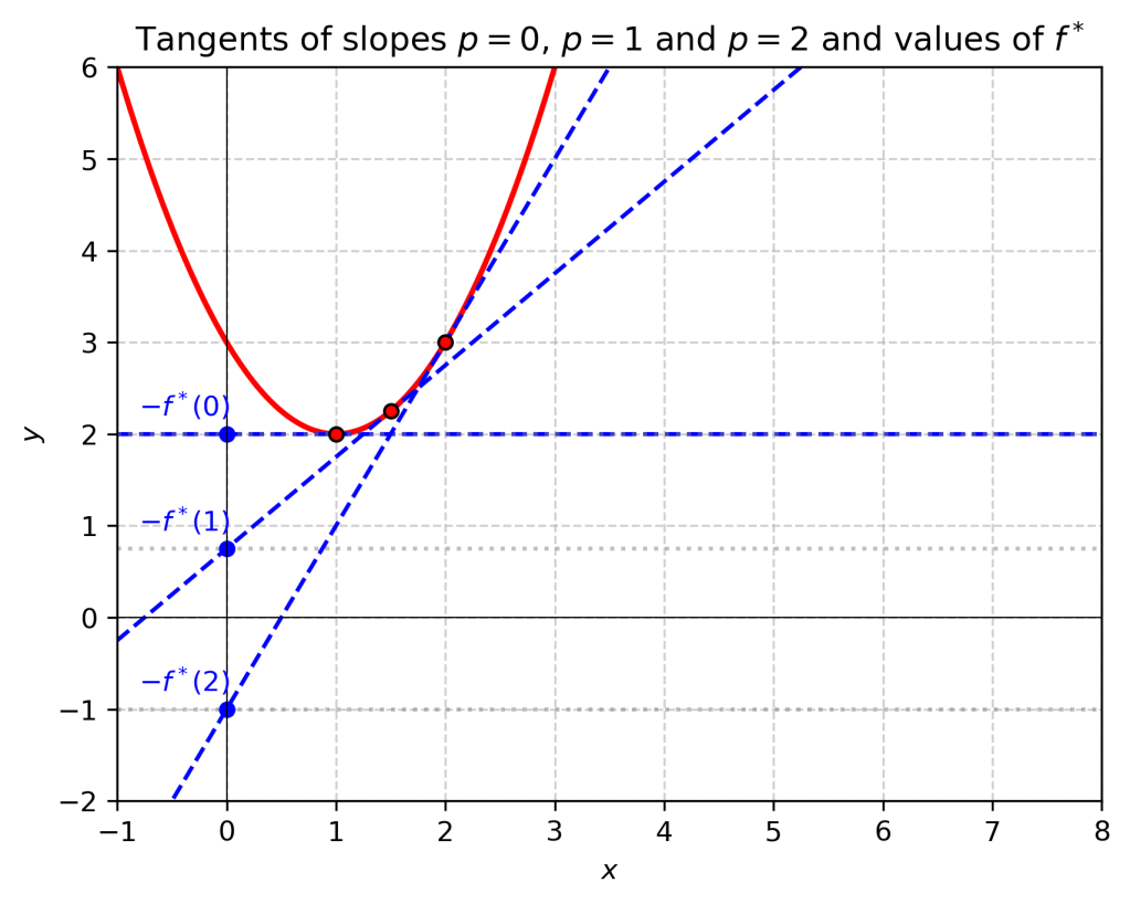
Namely, given a slope $p$ , we start by identifying the point $x$ such that $p=f'(x)$ . You can think of this operation as parallel-transporting a line with slope $p$ in the direction of the $y-$ axis starting from $y=-\infty$ . Assuming that $p\in\textrm{Im\ }f'$ , there will be a first point of contact with the graph of $f$ . At this point, the graph is tangent to the line. We will encode this information by recording the point of intersection with the $y$ – axis; more precisely, if our line has equation $y=px+b$ , we define $f^*(p)=-b$ . The knowledge of the function $f^*$ is tantamount to the knowledge of all the tangents to our graph: our original graph is their (uniquely defined) envelope. The function $f^*$ is called the Legendre transform of $f$ . In the figure below, the values of the transform of the function $f(x)=x^2-2x+3$ at $p=0, \, p=1$ and $p=2$ are represented.

It is easy to derive an explicit formula for $f^*$ . Given $p$ , we need to solve for $x=x(p)$ in the equation

$p=f'(x).$

The equation of the tangent is $y-f(x(p))=p(x-x(p))$ . Its $y$ -intercept is $b(p)=f(x(p))-px(p)$ . Finally,

$f^*(p)=-b(p)=px(p)-f(x(p))\qquad\qquad (1)$ .

This new function $f^*$ is convex. Indeed, a simple computation shows that

$\displaystyle{(f^*)''(p)=\frac 1{f''(x(p))}>0}$ .

From formula $(1)$ it follows that, given $x$ , we have

$f(x)=p(x)x-f^*(p(x)),$

where, as before, $f'(x)=p$ . The formula above reveals that $f=(f^*)^*$ , (i.e. the transformation is involutive), since

$\displaystyle{\frac{df^*(p)}{dp}=x(p)+p\frac{dx}{dp}-f'(x(p))\frac{dx}{dp}=x(p)+\frac{dx}{dp}\left[p-f'(x(p))\right]=x(p)}$

There is another way to look at this. For fixed $p$ in the range of $f'$ , the condition $p=f'(x)$ yields the (unique) critical point of the concave function $x\to px-f(x)$ . This point is a global maximum. Thus,

$f^*(p)=\max\limits_{x}\,(px-f(x)).\qquad\qquad (2)$ .

The latter equation implies the well-known Young’s inequality:

$f^*(p)+f(x)\ge px, \qquad\qquad (3)$

valid for any $x,p$ . Equality takes place when $x,p$ are linked by the relation $p=f'(x)$ .

Examples: If $f(x)=\frac{x^2}{2}$ , $f^*(p)=\frac{p^2}{2}$ . More generally, if $f(x)=\frac{x^{\alpha}}{\alpha}$ with $\alpha>1$ for $x>0$ , then $f^*(p)=\frac{p^{\beta}}{\beta}$ , where $1/\alpha+1/\beta=1$ . If $f(x)=e^x$ , then $f^*(p)=p\ln p -p$ , etc.

Generalizations

So far, we have assumed that our function $f$ is twice differentiable, with $f''(x)>0$ in its domain. However, the following slight modification of $(2)$ ,

$f^*(p)=\sup\limits_{x}\,(px-f(x))\qquad (4)$

is meaningful for any real $p$ and any function $f$ if we accept the values $\pm\infty$ in the range of $f^*$ . The resulting function $f^*$ , being the supremum of a family of linear functions, is convex on its domain. Definition $(4)$ , however, is not completely satisfactory for non-convex functions, as it loses information about the original function. However, for a convex function defined on $\mathbb{R}$ , $f^*$ encodes all the information about $f$ and, moreover, $f^{**}=f$ , a fact known as the Fenchel-Moreau theorem, [3]. Namely,

$f(x)=\sup\limits_{p}\,(px-f^{*}(p))\qquad (5)$ ,

which can be thought as a representation of $f$ as the envelope of its tangents. For convex functions defined on some domain $D\neq\mathbb{R}$ , an extra technical condition is needed on $f$ for $(5)$ to hold, namely lower semicontinuity, which is equivalent to the closedness of its epigraph. It is easy to see that this is a necessary condition for $(5)$ to hold. Indeed, $(5)$ furnishes a representation of the epigraph of $f$ as an intersection of closed half-planes, hence necessarily closed.

In the context of Convex Analysis, the more general transformation given by $(4)$ is called the Fenchel transform (or Fenchel-Legendre transform) and the more general inequality $(3)$ is called the Fenchel inequality (or Fenchel-Young inequality).

Thus, the transformation can be applied to a piece-wise linear, convex function. For instance, if $f$ is a linear function, $f(x)=ax+b$ , then clearly $f^*$ is finite only for $p=a$ , with $f^*(a)=b$ . If $f$ is made of two linear functions, $f(x)=a_1x+b_1$ when $x\le x_0$ and $f(x)=a_2x+b_2$ when $x\ge x_0$ , with $a_1<a_2$ and $a_1x_0+b_1=a_2x_0+b_2$ , then $f^*$ is finite only for $p\in [a_1,a_2]$ , where it is linear and ranges from $-b_1$ to $-b_2$ . In general, to each “corner” of a polygonal graph there corresponds a segment on the graph of $f^*$ , [2].

The generalization to functions $f:\mathbb{R}^n\to\mathbb{R}$ is straightforward. Under the smoothness and strict convexity assumption

$\displaystyle{\left(\frac{\partial^2f}{\partial x_i\partial x_j}\right)\succ 0}$ ,

the mapping $D: x\to df(x,\cdot)$ is one-to-one. If $p$ is the vector representing $df(x,\cdot)$ via the standard Euclidean structure, we define the Legendre transform by

$f^*(p)=\langle p, x\rangle-f(x), \qquad p\in \textrm{Im\ }D$ ,

where $\langle \cdot,\cdot\rangle$ denotes the inner product. Much like in the one-dimensional case, the previous definition is equivalent to

$f^*(p)=\max\limits_{x}\,(\langle p, x\rangle-f(x))$ .

Finally, we relax the smoothness and strict convexity assumptions and arrive at the most general definition

$f^*(p)=\sup\limits_{x}\,(\langle p, x\rangle-f(x))\qquad (5)$ ,

where now $f$ is merely convex and $f^*:\mathbb{R}^n\to (-\infty,+\infty]$ . The Fenchel-Moreau theorem holds without modifications under the extra assumption of lower semicontinuity of $f$ if it is not defined on all of $\mathbb{R}^n$ .

One can also consider “partial” Legendre transforms, i.e. transforms relative to some of the variables. Thus if $g:\mathbb{R}^2\to\mathbb{R}$ is a function of two variables, one can consider its transform with respect to the first variable,

$f_1^*(p_1,x_2)=\sup\limits_{x_1}\,( p_1 x_1-f(x_1,x_2))$ .

For smooth, strictly convex functions and fixed $x_2$ , the supremum is achieved at the (unique) $x_1$ defined by

$\displaystyle{p_1=\frac{\partial f}{\partial x_1}}$ .

The transform can be further generalized to functions on manifolds, but given the fact that a manifold does not have a global linear structure, the duality is established locally, between functions on the tangent bundle $TM$ and their “conjugates” or “dual” on the cotangent bundle $T^*M$ . Namely, the transform connects functions of $(x,v)$ with functions of $(x,p)$ , where $v\in T_xM$ and $p\in T^*_xM$ .

Applications

A) Clairaut’s differential equation

A standard example of ODE not solved for the derivative $y'$ is Clairaut’s equation

$y=xy'-f(y')$ .

It clearly admits the family of straight lines $y=px-f(p)$ as solutions. The envelope of the family is a singular solution satisfying $y=px-f(p)$ and $x=f'(p)$ . But these are precisely the relations defining the Legendre transform of $f$ . We conclude that, for convex $f$ , the singular solution of Clairaut equation is its Legendre transform.

B) Hamiltonian Mechanics from Lagrangian Mechanics.

For many Physics, Applied Math, and Engineering students, this is their first introduction to the Legendre transform. The Lagrangian of a mechanical system $L(q,\dot{q},t)$ on its configuration space (a differentiable, Riemannian manifold) completely describes the system. The actual path $q(t)$ joining two states $(t_1,q_1)$ and $(t_2,q_2)$ is an extremal of the action functional,

$S[q]=\displaystyle{\int\limits_{t_1}^{t_2}} L(q,\dot{q},t)\,dt$

(Hamilton’s principle) and therefore satisfies Euler-Lagrange second order differential equations

$\displaystyle{\frac{d}{dt}\frac{\partial L}{\partial \dot{q}}-\frac{\partial L}{\partial q}=0}$ .

Te geometry of the configuration space is intimately connected to the Physics. Thus, holonomic constraints are built into the manifold, the kinetic energy is nothing but the Riemannian metric on the manifold, geodesics relative to this metric represent motion “by inertia”, etc. The alternative Hamiltonian description reveals connections to a different geometry and is introduced as follows. Assuming that the Lagrangian is strictly convex in the generalized velocities $\dot{q}$ ,

$\displaystyle{\left(\frac{\partial^2L}{\partial \dot q_i\partial\dot q_j}\right)\succ 0},$

we introduce the Hamiltonian of the system as the Legendre transform of the Lagrangian with respect to $\dot{q}$ :

$\displaystyle{H(p,q,t)=\langle p,\dot{q}\rangle -L(q,\dot{q},t)}$ ,

where $\displaystyle{p=\frac{\partial L}{\partial \dot{q}}}$ is the generalized momentum, an element of the cotangent fiber at $q$ . Since

$\displaystyle{dH=\langle\dot{q},dp\rangle +\langle p,d\dot{q}\rangle-\langle\frac{\partial L}{\partial q},dq\rangle-\langle\frac{\partial L}{\partial \dot{q}},d\dot{q}\rangle-\frac{\partial L}{\partial t}dt}$

$\displaystyle{\,\,\, =\langle\dot{q},dp\rangle-\langle\dot{p},dq\rangle-\frac{\partial L}{\partial t}dt}$

it follows that $(p,q)$ satisfy the first order Hamiltonian system:

$\displaystyle{\dot{p}=-\frac{\partial H}{\partial q}};\qquad \displaystyle{\dot{q}=\frac{\partial H}{\partial p}}$

The space $\{(p,q)\}$ is called the phase space, and the Hamiltonian function equips it with a remarkable symplectic structure. The Hamiltonian flow (if $H$ does not depend on time) is a one-parameter subgroup of the group of symplectomorphisms of the phase space. A straightforward consequence is Liouville’s Theorem on the preservation of the phase volume (a cornerstone of Statistical Mechanics) . The Lagrangian approach has, however, certain advantages including: a) it is easier to deal with constraints, even non-holonomic via Lagrange multipliers; b) it is easier to track conserved quantities via Noether’s theorem, c) non-conservative forces can be incorporated, etc.

It is worth noticing that the above “Hamiltonization” applies to general variational problems, not just to the problem related to mechanical systems. In the case of mechanical systems, the part of the Lagrangian depending on $\dot q$ is usually a positive definite quadratic function (the kinetic energy of the system) hence convex. The transform of a quadratic form is especially simple: it is just another quadratic form of the conjugate variable. For instance, the Lagrangian of a simple mass-spring system, assuming that the spring is linear and $q$ represents the deviation of the mass from equilibrium is

$L(q,\dot q)=\displaystyle{\frac 1{2}m\dot q^2-\frac 1{2}m q^2}$

and the Hamiltonian is

$H(p,q)=\displaystyle{\frac {p^2}{2m}+\frac 1{2}m q^2}$

and represents the total energy of the system. That is the case whenever the Lagrangian is quadratic on velocities, the system is conservative and the constraints are time-independent.

C) Thermodynamic potentials

Yet another early use of the transform was in Thermodynamics, as a way to switch between potentials according to the most convenient independent parameters.

According to the first principle of Thermodynamics (energy conservation), there exists a function of state $U$ (internal energy) such that, for any thermodynamical system undergoing an infinitesimal change of state,

$\displaystyle{dU=\delta Q+\delta W+\sum_i\mu_idN_i}$ ,

where $\delta Q$ represent the heat (thermal energy) added to the system, $\delta W$ is the work of the surroundings on the system and the last sum above accounts for the energy added to the system by means of particle exchange. Here, $dN_i$ is the amount of particles of the $i$ -th type added to the system, and $\mu_i$ the corresponding chemical potential. The relevant fact here is that $dU$ is an actual differential, whereas the rest of the terms are just differential forms in the configuration space of the system. The term $\delta W$ is in general a differential form $\sum p_idq_i$ involving intensive ( $p_i$ ) and conjugate extensive variables $dq_i$ . Thus, for example, in the case of a gas expanding/compressing against the environment, the work done on the gas is $\delta W=-p_{ext}dV$ , where $dV$ is the infinitesimal change of volume and $p_{ext}$ is the external pressure. Moreover, according to the second principle, for reversible processes the form $\delta Q$ admits an integrating factor $\frac 1{T}$ , namely there is a function of state called entropy $S$ such that

$\displaystyle{dS= \frac{\delta Q}{T}}$

Putting all together, for an infinitesimal, reversible (hence quasi-static) process undergone by a gas we get

$\displaystyle{dU=TdS-pdV+\sum_i\mu_idN_i}\qquad (6)$

where $p=p_{ext}$ is the pressure of the gas in equilibrium with its surroundings.

While $U$ accounts for the total energy of the system, related state functions accounting for different manifestations of energy may result more convenient for particular experimental or theoretical scenarios. For instance, many chemical reactions occur at constant pressure in lab conditions. In such cases, it is convenient to include a term representing the work needed to push aside the surroundings to occupy volume $V$ at pressure $p$ , namely we define the enthalpy of the system as

$H=U+pV$ .

Given that, thanks to $(6)$ we have $\partial U/\partial V=-p$ , $H$ is nothing but (minus) the Legendre transform of $U$ with respect to $V$ , that is,

$H(S,p)=-U^*(S,p)$ .

(in Thermodynamics, the transform is usually defined with opposite sign so there is no “minus” in the previous formula. A possible reason is that one prefers all forms of energy to increase/decrease in agreement). Assuming for simplicity that $dN=0$ we have

$dH=dU+pdV+Vdp=TdS-pdV+pdV+Vdp=TdS+Vdp$

and, therefore, at constant pressure, $dH=TdS=\delta Q$ . Thus, the change of enthalpy determines if a given chemical reaction is exothermic or endothermic. Moreover, $\partial H/\partial S=T$ and $\partial H/\partial p=V$ .

In a similar fashion, one can consider the (opposite of) Legendre transform of $U$ with respect to entropy,

$F=U-TS$ ,

called (Helmholtz) free energy. A similar computation shows that

$dF=-SdT-pdV$ ,

thus we can think of $dF$ as the pressure-volume work on the system under fixed temperature.

Yet another thermodynamic potential, the Gibbs free energy, is a measure of the maximum reversible work a system can perform at constant pressure (P) and temperature (T), excluding expansion work. It is useful to determine if a given process occurs spontaneously (e.g., chemical reactions, phase transitions) and equilibrium conditions.

Bibliography

[1] Legendre, A. M., “Mémoire sur l’intégration de quelques équations aux différences partielles.” Histoire de l’Académie Royale des Sciences, 1789, pp. 309–351.

[2] Arnold, V. I. “Mathematical Methods of Classical Mechanics”, 2nd Edition, Graduate Texts in Mathematics (60), 1989.

[3] Boyd, Stephen P. and Vandenberghe, L. “Convex Optimization“. Cambridge University Press, 2004.

Math Bites

by Guillermo Reyes, PhD

thermodynamic-potentials

The Legendre transform and some applications

Generalizations

Applications

Bibliography