The structure of the real line is deceptively intricate. Rational and irrational numbers are densely interwoven, yet they differ fundamentally—not just in their arithmetic properties, but in how they can be approximated. Even the rationals themselves possess a rich, hierarchical organization, elegantly captured by the Stern-Brocot tree.
If you take a course on Real Analysis where these matters are looked at in some detail, or an Algebra course where extensions of the rational field are considered (say, a course on Galois theory), you encounter the concepts of algebraic and transcendental numbers. Rational numbers can be thought as the ones solving a linear equation with integer coefficients, . A natural generalization leads us to the definition of algebraic numbers as real numbers satisfying a polynomial equation of the form with integer coefficients . The degree of an algebraic number is the lowest degree of a polynomial with integer coefficients having the given number as a root. Such polynomial has to be irreducible in , otherwise the said number would be a root of a lower degree polynomial. Real numbers which are not algebraic are called transcendental. Clearly, all rational numbers are algebraic, and all transcendental numbers are irrational.
The idea of the existence of transcendental numbers goes back to Leibniz, but the first to prove it, by giving a concrete example, was J. Liouville in papers from 1844 and 1851, [1] & [2]. It is often the case that when transcendental numbers are presented, the examples provided include , , and the Euler-Mascheroni constant or Apéry’s constant are mentioned as candidates (it is not even known if those are irrational). Proving that or are transcendental was accomplished by Hermite and Lindemann in the second half of the XIX century, and their proofs are far from elementary and can hardly be motivated and put in simple terms.
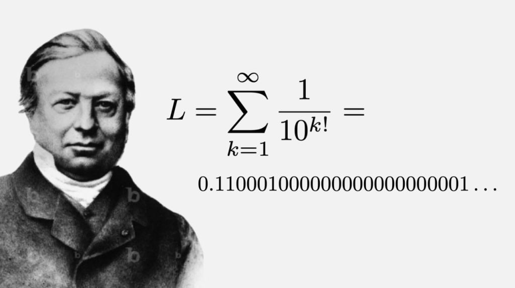
In contrast, Liouville’s constant has a very simple structure and the proof of its transcendency is completely elementary. It is defined as the number
,
that is, the number where the “ones” appear at positions given by the factorials, after the decimal point. Not being periodic, is clearly irrational.
Here is the reason why is transcendental: it can be approximated “too well” by the partial sums of the series, contradicting a result proved by Liouville, whose (very simple) proof is given below. The statement of the result, which we accept for the time being, is as follows.
Theorem [1] : Let be an irrational algebraic number of degree (i.e., is a root of an irreducible polynomial of degree with integer coefficients). Then there exists a constant such that for all rational numbers (with ) we have
.
(in words, algebraic numbers are not “too close” to rationals, in the sense that the rate of convergence of sequences of rationals with increasing denominators is limited by the degree of the given algebraic number). Formula should be contrasted with the well known fact that the continued fraction convergents of any irrational number satisfy
.
Liouville’s constant violates the theorem
The partial sums are rational numbers with denominator . It is clear that
On the other hand, if were algebraic of degree , we would have, according to Liouville’s Theorem,
But relations and clearly contradict each other for large . Indeed, for large enough , we have
,
since . Thus, is transcendental.
A proof of Liouville’s Theorem
Proof: By definition, there exists an irreducible polynomial in
with . If is a rational number in lowest terms (, then is a non-zero integer,
and therefore
.
Next, we relate to via the Mean Value Theorem,
for some between and . If we fix an interval around , that is, if we assume, say, , then and the previous estimate entails
.
The assertion follows with .
Final Remarks
During the time of Liouville and Hermite, transcendental numbers appeared rare and exotic, requiring ingenious proofs to isolate even a handful of examples. Yet just a few decades later, in 1874, Cantor demonstrated that, in fact, almost all real numbers are transcendental. What seemed like a hunt for “needles in a haystack” turned out to be a realization that the “haystack” was almost entirely made of “needles.” His proof, however, was non-constructive—relying not on explicit examples but on the abstract principles of cardinality and the countability of algebraic numbers.
Here is a question worth pondering: If almost all numbers are transcendental, why do the ones we encounter so rarely reflect that? Part of the answer to this question is probably that humans think algorithmically. We are drawn to numbers we can compute, describe, or construct. Most numbers are not describable.
The apparent simplicity of Liouville’s constant is deceptive—a trick of human intuition. What makes it seem simple is merely the ease of describing its decimal representation. By contrast, a number like might appear ‘chaotic’ in its decimal expansion, yet it is fundamentally structured: as a quadratic irrational, its continued fraction is perfectly periodic,
.
The same applies, for instance, to the golden ratio, again a quadratic irrational with a very simple continued fraction representation, etc. This reveals a deeper truth: our perception of mathematical simplicity often depends on the representation we choose, not the object itself.
I hope you enjoyed this dive into Liouville’s constant — its deceptively tidy decimal mask is, after all, a very human kind of charm.
[2] Liouville, J. (1851), “Sur des classes très étendues de quantités dont la valeur n’est ni algébrique, ni même réductible à des irrationnelles algébriques”, Journal de Mathématiques Pures et Appliquées, 16, 133–142. https://www.numdam.org/item/JMPA_1851_1_16__133_0.pdf
The Legendre transform has its origins in the work of A.M. Legendre [1], where it was introduced to recast a first order PDE into a more convenient form. It gained significance around 1830 with the reformulation of Lagrangian mechanics carried out by W. R. Hamilton by replacing the “natural” configuration space by the so called phase space with its rich symplectic structure [2] and as a central tool in Hamilton-Jacobi theory. In the late 19th century, it was used in Thermodynamics (Gibbs, Maxwell) as a way of switching between different thermodynamic potentials. With the development of Convex Analysis and Optimization in the 20th century, its central role in providing so called dual representations of functions, problems, etc. became apparent, [3].
From a high level point of view, the transform establishes a link between a function of a variable belonging to or a more general topological vector space and its “dual” or “conjugate” function, defined on the dual space of linear forms. From a more practical perspective, it can be understood as an alternative way of encoding the information contained in a function. In that sense, it is very similar to other transforms like the Fourier series/transform and the Laplace transform. The Fourier series, for instance, encodes the information about the given (periodic) function in the form of a sequence of “amplitudes” corresponding to the different “modes”. The Fourier transform furnishes a similar integral representation for non-periodic functions, where this time different “modes” or “frequencies” form a continuum. Both the series and the transform provide a spectral representation of the function.
Suppose we are given a convex real function of one real variable. Let us assume for simplicity that is twice differentiable and for all . Typical examples are quadratic functions with , exponential functions with , the function , etc.
Since , is a strictly increasing (hence one-to-one) function. Such correspondence allows to identify with the value of the slope of at that point, . In other words, can be used as a new independent variable. At this point, one might be tempted to use the function , where (or ) as an alternative representation of . This is, no doubt, a possible choice. However, a little extra work provides a function that has the following pleasant additional property: if the procedure is applied twice we recover the original function, . The transformation is what is called involutive (an involution).
Namely, given a slope , we start by identifying the point such that . You can think of this operation as parallel-transporting a line with slope in the direction of the axis starting from . Assuming that , there will be a first point of contact with the graph of . At this point, the graph is tangent to the line. We will encode this information by recording the point of intersection with the – axis; more precisely, if our line has equation , we define . The knowledge of the function is tantamount to the knowledge of all the tangents to our graph: our original graph is their (uniquely defined) envelope. The function is called the Legendre transform of . In the figure below, the values of the transform of the function at and are represented.
It is easy to derive an explicit formula for . Given , we need to solve for in the equation
The equation of the tangent is . Its -intercept is . Finally,
.
This new function is convex. Indeed, a simple computation shows that
.
From formula it follows that, given , we have
where, as before, . The formula above reveals that , (i.e. the transformation is involutive), since
There is another way to look at this. For fixed in the range of , the condition yields the (unique) critical point of the concave function . This point is a global maximum. Thus,
.
The latter equation implies the well-known Young’s inequality:
valid for any . Equality takes place when are linked by the relation .
Examples: If , . More generally, if with for , then , where . If , then , etc.
Generalizations
So far, we have assumed that our function is twice differentiable, with in its domain. However, the following slight modification of ,
is meaningful for any real and any function if we accept the values in the range of . The resulting function , being the supremum of a family of linear functions, is convex on its domain. Definition , however, is not completely satisfactory for non-convex functions, as it loses information about the original function. However, for a convex function defined on , encodes all the information about and, moreover, , a fact known as the Fenchel-Moreau theorem, [3]. Namely,
,
which can be thought as a representation of as the envelope of its tangents. For convex functions defined on some domain , an extra technical condition is needed on for to hold, namely lower semicontinuity, which is equivalent to the closedness of its epigraph. It is easy to see that this is a necessary condition for to hold. Indeed, furnishes a representation of the epigraph of as an intersection of closed half-planes, hence necessarily closed.
In the context of Convex Analysis, the more general transformation given by is called the Fenchel transform (or Fenchel-Legendre transform) and the more general inequality is called the Fenchel inequality (or Fenchel-Young inequality).
Thus, the transformation can be applied to a piece-wise linear, convex function. For instance, if is a linear function, , then clearly is finite only for , with . If is made of two linear functions, when and when , with and , then is finite only for , where it is linear and ranges from to . In general, to each “corner” of a polygonal graph there corresponds a segment on the graph of , [2].
The generalization to functions is straightforward. Under the smoothness and strict convexity assumption
,
the mapping is one-to-one. If is the vector representing via the standard Euclidean structure, we define the Legendre transform by
,
where denotes the inner product. Much like in the one-dimensional case, the previous definition is equivalent to
.
Finally, we relax the smoothness and strict convexity assumptions and arrive at the most general definition
,
where now is merely convex and . The Fenchel-Moreau theorem holds without modifications under the extra assumption of lower semicontinuity of if it is not defined on all of .
One can also consider “partial” Legendre transforms, i.e. transforms relative to some of the variables. Thus if is a function of two variables, one can consider its transform with respect to the first variable,
.
For smooth, strictly convex functions and fixed , the supremum is achieved at the (unique) defined by
.
The transform can be further generalized to functions on manifolds, but given the fact that a manifold does not have a global linear structure, the duality is established locally, between functions on the tangent bundle and their “conjugates” or “dual” on the cotangent bundle . Namely, the transform connects functions of with functions of , where and .
Applications
A)Clairaut’s differential equation
A standard example of ODE not solved for the derivative is Clairaut’s equation
.
It clearly admits the family of straight lines as solutions. The envelope of the family is a singular solution satisfying and . But these are precisely the relations defining the Legendre transform of . We conclude that, for convex , the singular solution of Clairaut equation is its Legendre transform.
B)Hamiltonian Mechanics from Lagrangian Mechanics.
For many Physics, Applied Math, and Engineering students, this is their first introduction to the Legendre transform. The Lagrangian of a mechanical system on its configuration space (a differentiable, Riemannian manifold) completely describes the system. The actual path joining two states and is an extremal of the action functional,
(Hamilton’s principle) and therefore satisfies Euler-Lagrange second order differential equations
.
Te geometry of the configuration space is intimately connected to the Physics. Thus, holonomic constraints are built into the manifold, the kinetic energy is nothing but the Riemannian metric on the manifold, geodesics relative to this metric represent motion “by inertia”, etc. The alternative Hamiltonian description reveals connections to a different geometry and is introduced as follows. Assuming that the Lagrangian is strictly convex in the generalized velocities ,
we introduce the Hamiltonian of the system as the Legendre transform of the Lagrangian with respect to :
,
where is the generalized momentum, an element of the cotangent fiber at . Since
it follows that satisfy the first order Hamiltonian system:
The space is called the phase space, and the Hamiltonian function equips it with a remarkable symplectic structure. The Hamiltonian flow (if does not depend on time) is a one-parameter subgroup of the group of symplectomorphisms of the phase space. A straightforward consequence is Liouville’s Theorem on the preservation of the phase volume (a cornerstone of Statistical Mechanics) . The Lagrangian approach has, however, certain advantages including: a) it is easier to deal with constraints, even non-holonomic via Lagrange multipliers; b) it is easier to track conserved quantities via Noether’s theorem, c) non-conservative forces can be incorporated, etc.
It is worth noticing that the above “Hamiltonization” applies to general variational problems, not just to the problem related to mechanical systems. In the case of mechanical systems, the part of the Lagrangian depending on is usually a positive definite quadratic function (the kinetic energy of the system) hence convex. The transform of a quadratic form is especially simple: it is just another quadratic form of the conjugate variable. For instance, the Lagrangian of a simple mass-spring system, assuming that the spring is linear and represents the deviation of the mass from equilibrium is
and the Hamiltonian is
and represents the total energy of the system. That is the case whenever the Lagrangian is quadratic on velocities, the system is conservative and the constraints are time-independent.
C)Thermodynamic potentials
Yet another early use of the transform was in Thermodynamics, as a way to switch between potentials according to the most convenient independent parameters.
According to the first principle of Thermodynamics (energy conservation), there exists a function of state (internal energy) such that, for any thermodynamical system undergoing an infinitesimal change of state,
,
where represent the heat (thermal energy) added to the system, is the work of the surroundings on the system and the last sum above accounts for the energy added to the system by means of particle exchange. Here, is the amount of particles of the -th type added to the system, and the corresponding chemical potential. The relevant fact here is that is an actual differential, whereas the rest of the terms are just differential forms in the configuration space of the system. The term is in general a differential form involving intensive () and conjugate extensive variables . Thus, for example, in the case of a gas expanding/compressing against the environment, the work done on the gas is , where is the infinitesimal change of volume and is the external pressure. Moreover, according to the second principle, for reversible processes the form admits an integrating factor , namely there is a function of state called entropy such that
Putting all together, for an infinitesimal, reversible (hence quasi-static) process undergone by a gas we get
where is the pressure of the gas in equilibrium with its surroundings.
While accounts for the total energy of the system, related state functions accounting for different manifestations of energy may result more convenient for particular experimental or theoretical scenarios. For instance, many chemical reactions occur at constant pressure in lab conditions. In such cases, it is convenient to include a term representing the work needed to push aside the surroundings to occupy volume at pressure , namely we define the enthalpy of the system as
.
Given that, thanks to we have , is nothing but (minus) the Legendre transform of with respect to , that is,
.
(in Thermodynamics, the transform is usually defined with opposite sign so there is no “minus” in the previous formula. A possible reason is that one prefers all forms of energy to increase/decrease in agreement). Assuming for simplicity that we have
and, therefore, at constant pressure, . Thus, the change of enthalpy determines if a given chemical reaction is exothermic or endothermic. Moreover, and .
In a similar fashion, one can consider the (opposite of) Legendre transform of with respect to entropy,
,
called (Helmholtz) free energy. A similar computation shows that
,
thus we can think of as the pressure-volume work on the system under fixed temperature.
Yet another thermodynamic potential, the Gibbs free energy, is a measure of the maximum reversible work a system can perform at constant pressure (P) and temperature (T), excluding expansion work. It is useful to determine if a given process occurs spontaneously (e.g., chemical reactions, phase transitions) and equilibrium conditions.
Bibliography
[1] Legendre, A. M., “Mémoire sur l’intégration de quelques équations aux différences partielles.”Histoire de l’Académie Royale des Sciences, 1789, pp. 309–351.
[2] Arnold, V. I. “Mathematical Methods of Classical Mechanics”, 2nd Edition, Graduate Texts in Mathematics (60), 1989.
[3] Boyd, Stephen P. and Vandenberghe, L. “Convex Optimization“. Cambridge University Press, 2004.
A slant asymptote for a real function of one real variable is a line with the property
,
where as . Geometrically, the graph of comes closer and closer to the line for large positive/negative values of . For the sake of simplicity, we will deal with asymptotes at , the other case being completely analogous. When we say that the asymptote is horizontal. A simple way to detect if a given function has a slant asymptote is by checking linearity at infinity, if the limit
is finite. If that is the case, the value of the limit is the slope of the asymptote, . The free term is then given by the limit
,
if the latter exists (and is finite). For rational functions of the form
where and are polynomials, the situation is much simpler. In order for to be linear at infinity, we need and, if that is the case, we perform long division which leads to
where and, therefore, the asymptote is just the quotient since
When , the fraction is superlinear at infinity.
All this is well known and usually taught in high school.
On the other hand, students are taught to find tangents to a given curve at a given point by means of derivatives. It turns out, however, that finding the tangent to a rational function at does not require derivatives at all. In order to understand this, we notice that is a tangent to at precisely when
with as . The last relation is very similar to except for the fact that now we are looking at instead of . Thus, if we could somehow come up with a relation like where now
,
the quotient would be the tangent.
As it happens, that is perfectly possible. All we need to do is divide the polynomials starting with the lowest powers (backwards), until we reach a “partial remainder” whose lowest degree is two or higher. Observe that the lowest degree of the divisor is necessarily zero (otherwise is undefined at ).
As an example, let us find the tangent to the graph of
at . Starting with the lowest degree, we have , with first partial remainder . In the next step, we add to the quotient, with a partial remainder . Since we are interested in the tangent line and is an infinitesimal of degree higher than one at zero, the division stops here and the equation of the tangent is . If we keep dividing, we get the Taylor polynomials of higher degree. For instance, the osculating parabola at is and so on.
Long division is taught at school starting with the highest powers. A possible reason is that long division of numbers proceeds by reducing the remainder at each step. If we replace the base in the decimal representation of numbers by , we arrive at the usual long division algorithms of polynomials, reducing the degree at each step. I would call this procedure “division at infinity”. In contrast, the above is an example of “division at zero”.
Finding the tangent to a rational function at a point different from zero can be reduced to the previous case. If, say, we need to find the tangent to at , all we need to do is set and express and as polynomials in and then finding the tangent at as before. Finally, we have to replace back by in the found equation of the tangent.
The above reveals a perfect symmetry between the problems of finding the asymptote and that of finding the tangent at . In some sense, we can say that an asymptote is a “tangent at infinity” and, I guess, that a tangent is an asymptote at a finite point. Both problems are algebraic in nature and can be solved without limit procedures, just by means of division (forward or backward).
More generally, for rational functions, being the simplest non-polynomial functions, finding their Taylor expansion at zero (and, by translation at any point) is a pure algebraic procedure. I believe this fact should be emphasized in high school and it could be used as a motivating example to introduce more general power expansions. As a matter of fact, Newton was inspired by the algorithm of long division for numbers to start experimenting with power series, not necessarily with integer powers. The image below shows a page from his “Method of Fluxions and Infinite Series”. The “backwards” long division of by is performed in order to get the power series expansion.
The differential of a quotient
Here is yet another example of “division at zero”.
When students are exposed to the differentiation rules, those are derived from the definition of derivative as the limit of the differential quotient. Thus for example to prove the rule of differentiation of a product we proceed as follows.
given that all the limits are assumed to exist. A similar computation can be done for the quotient. It should be noted, however, that a little algebraic trick has to be used in both cases to make the derivatives of the individual factors appear explicitly. No big deal, but a bit artificial. And, importantly, not the way the founders of Infinitesimal Calculus arrived at these rules.
To help intuition, the product rule is often presented in the form
,
and the last term is ignored in the last equality as being a quadratic infinitesimal (in Leibniz’ terminology, the last equality is actually an “adequality”, a term coined by Fermat). Without a doubt, the latter derivation, albeit not meeting the modern standards of rigor, reveals the reason for the presence of the “mixed” terms and the general structure of the formula. Moreover, no algebraic tricks are required. The formula follows in a straightforward manner.
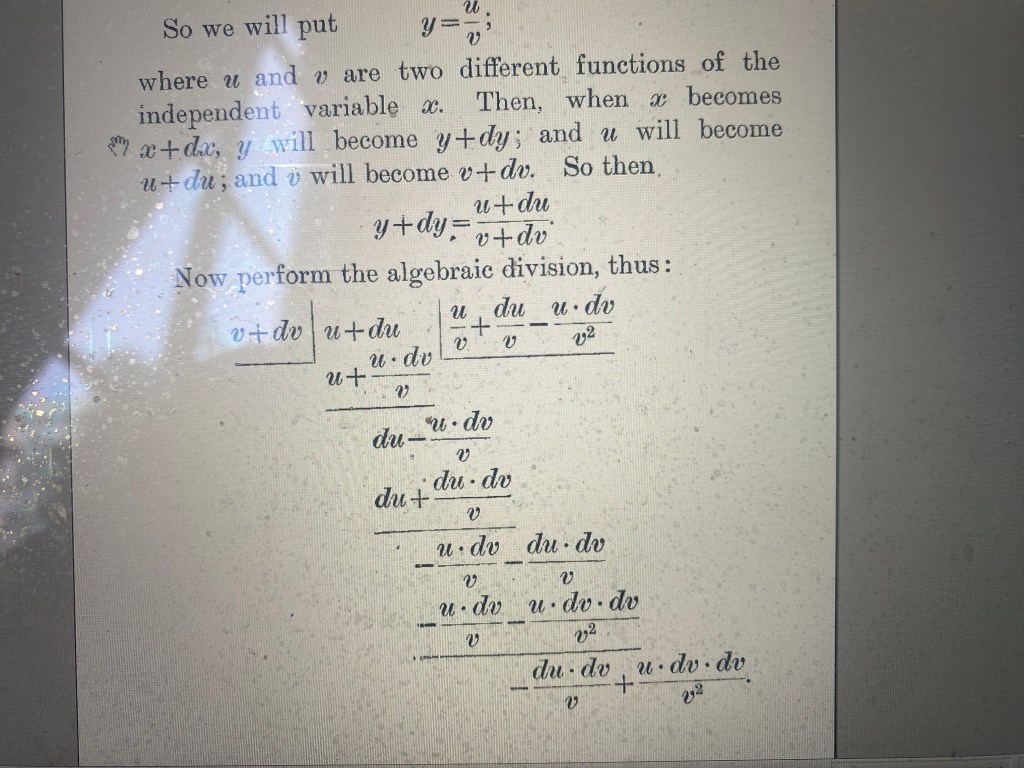
A similar derivation of the quotient rule involves “division at zero”. Here is the derivation in the book “Calculus made easy” by Silvanus Thompson, from 1910.
Observe that the operation has been stopped when the remainder is a quadratic infinitesimal. The conclusion of the computation is the familiar rule


![\mathbb{Z}[x]](https://s0.wp.com/latex.php?latex=%5Cmathbb%7BZ%7D%5Bx%5D&bg=ffffff&fg=444444&s=0&c=20201002)


 belonging to
  or a more general topological vector space and its “dual” or “conjugate” function, defined on the dual space of linear forms. From a more practical perspective, it can be understood as an alternative way of encoding the information contained in a function. In that sense, it is very similar to other transforms like the Fourier series/transform and the Laplace transform. The Fourier series, for instance, encodes the information about the given (periodic) function in the form of a sequence of “amplitudes” corresponding to the different “modes”. The Fourier transform furnishes a similar integral representation for non-periodic functions, where this time different “modes” or “frequencies” form a continuum. Both the series and the transform provide a spectral representation of the function.
 is twice differentiable and
  for all
  with
with  , exponential functions
  with
with  , the function
  , etc.
 is a strictly increasing (hence one-to-one) function. Such correspondence allows to identify
  . In other words,
  can be used as a new independent variable. At this point, one might be tempted to use the function
  , where
  ) as an alternative representation of
  that has the following pleasant additional property: if the procedure is applied twice we recover the original function,
  . The transformation
  is what is called involutive (an involution).
 axis starting from
  . Assuming that
  , there will be a first point of contact with the graph of
  – axis; more precisely, if our line has equation
  , we define
  . The knowledge of the function
  at
at  and
and  are represented.
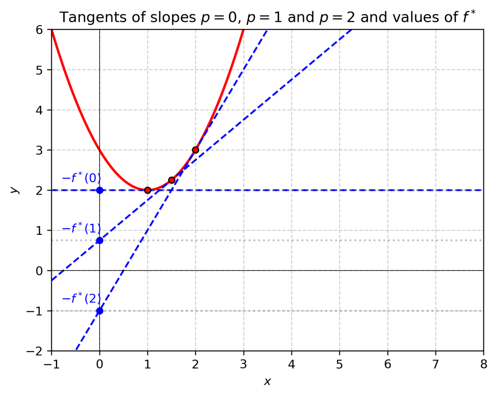
 in the equation
 . Its
. Its  . Finally,
 .
. .
.
 . The formula above reveals that
  , (i.e. the transformation is involutive), since
![\displaystyle{\frac{df^*(p)}{dp}=x(p)+p\frac{dx}{dp}-f'(x(p))\frac{dx}{dp}=x(p)+\frac{dx}{dp}\left[p-f'(x(p))\right]=x(p)}](https://s0.wp.com/latex.php?latex=%5Cdisplaystyle%7B%5Cfrac%7Bdf%5E%2A%28p%29%7D%7Bdp%7D%3Dx%28p%29%2Bp%5Cfrac%7Bdx%7D%7Bdp%7D-f%27%28x%28p%29%29%5Cfrac%7Bdx%7D%7Bdp%7D%3Dx%28p%29%2B%5Cfrac%7Bdx%7D%7Bdp%7D%5Cleft%5Bp-f%27%28x%28p%29%29%5Cright%5D%3Dx%28p%29%7D&bg=ffffff&fg=444444&s=0&c=20201002)
 . This point is a global maximum. Thus,
 .
.
 . Equality takes place when
  ,
,  . More generally, if
  with
with  for
for  , then
  , where
  . If
. If  , then
  , etc.
 in the range of
  , however, is not completely satisfactory for non-convex functions, as it loses information about the original function. However, for a convex function defined on
  ,
,  , a fact known as the Fenchel-Moreau theorem, [3]. Namely,
 ,
, , an extra technical condition is needed on
  to hold, namely lower semicontinuity, which is equivalent to the closedness of its epigraph. It is easy to see that this is a necessary condition for
  , then clearly
  , with
  . If
. If  when
when  and
and  when
when  , with
  and
and  , then
 ![p\in [a_1,a_2]](https://s0.wp.com/latex.php?latex=p%5Cin+%5Ba_1%2Ca_2%5D&bg=ffffff&fg=444444&s=0&c=20201002) , where it is linear and ranges from
, where it is linear and ranges from  to
to  . In general, to each “corner” of a polygonal graph there corresponds a segment on the graph of
  is straightforward. Under the smoothness and strict convexity assumption
 ,
,  is one-to-one. If
  via the standard Euclidean structure, we define the Legendre transform by
 ,
, denotes the inner product. Much like in the one-dimensional case, the previous definition is equivalent to
  .
. ,
,![f^*:\mathbb{R}^n\to (-\infty,+\infty]](https://s0.wp.com/latex.php?latex=f%5E%2A%3A%5Cmathbb%7BR%7D%5En%5Cto+%28-%5Cinfty%2C%2B%5Cinfty%5D&bg=ffffff&fg=444444&s=0&c=20201002) . The Fenchel-Moreau theorem holds without modifications under the extra assumption of lower semicontinuity of
. The Fenchel-Moreau theorem holds without modifications under the extra assumption of lower semicontinuity of  is a function of two variables, one can consider its transform with respect to the first variable,
 .
. , the supremum is achieved at the (unique)
  defined by
  .
. and their “conjugates” or “dual” on the cotangent bundle
  . Namely, the transform connects functions of
  with functions of
  , where
  and
and  .
. is Clairaut’s equation
 .
. as solutions. The envelope of the family is a singular solution satisfying
  . But these are precisely the relations defining the Legendre transform of
  on its configuration space (a differentiable, Riemannian manifold) completely describes the system. The actual path
  joining two states
  and
and  is an extremal of the action functional,
![S[q]=\displaystyle{\int\limits_{t_1}^{t_2}} L(q,\dot{q},t)\,dt](https://s0.wp.com/latex.php?latex=S%5Bq%5D%3D%5Cdisplaystyle%7B%5Cint%5Climits_%7Bt_1%7D%5E%7Bt_2%7D%7D++L%28q%2C%5Cdot%7Bq%7D%2Ct%29%5C%2Cdt&bg=ffffff&fg=444444&s=0&c=20201002)
 .
.  ,
,
 ,
, is the generalized momentum, an element of the cotangent fiber at
  . Since

 satisfy the first order Hamiltonian system:
 is called the phase space, and the Hamiltonian function equips it with a remarkable symplectic structure. The Hamiltonian flow (if
  does not depend on time) is a one-parameter subgroup of the group of symplectomorphisms of the phase space. A straightforward consequence is Liouville’s Theorem on the preservation of the phase volume (a cornerstone of Statistical Mechanics) . The Lagrangian approach has, however, certain advantages including: a) it is easier to deal with constraints, even non-holonomic via Lagrange multipliers; b) it is easier to track conserved quantities via Noether’s theorem, c) non-conservative forces can be incorporated, etc.
 is usually a positive definite quadratic function (the kinetic energy of the system) hence convex. The transform of a quadratic form is especially simple: it is just another quadratic form of the conjugate variable. For instance, the Lagrangian of a simple mass-spring system, assuming that the spring is linear and

 (internal energy) such that, for any thermodynamical system undergoing an infinitesimal change of state,
 ,
, represent the heat (thermal energy) added to the system,
  is the work of the surroundings on the system and the last sum above accounts for the energy added to the system by means of particle exchange. Here,
  is the amount of particles of the
  -th type added to the system, and
  the corresponding chemical potential. The relevant fact here is that
  is an actual differential, whereas the rest of the terms are just differential forms in the configuration space of the system. The term
  involving intensive (
 ) and conjugate extensive variables
  . Thus, for example, in the case of a gas expanding/compressing against the environment, the work done on the gas is
  , where
  is the infinitesimal change of volume and
  is the external pressure. Moreover, according to the second principle, for reversible processes the form
  , namely there is a function of state called entropy
  such that

 is the pressure of the gas in equilibrium with its surroundings.
  at pressure
  .
. we have
  ,
,  .
.  we have
 . Thus, the change of enthalpy determines if a given chemical reaction is exothermic or endothermic. Moreover,
  and
and  .
. ,
, ,
, as the pressure-volume work on the system under fixed temperature.
  with the property
 ,
, as
as  . Geometrically, the graph of
  , the other case being completely analogous. When
  we say that the asymptote is horizontal. A simple way to detect if a given function has a slant asymptote is by checking linearity at infinity,
  if the limit
 . The free term
  is then given by the limit
 ,
,
 and
and  are polynomials, the situation is much simpler. In order for
  and, if that is the case, we perform long division which leads to
 and, therefore, the asymptote is just the quotient
 , the fraction is superlinear at infinity.
  does not require derivatives at all. In order to understand this, we notice that
  is a tangent to
  at
at 
 as
as  . The last relation is very similar to
  . Thus, if we could somehow come up with a relation like
  ,
, 
 ,
,  with first partial remainder
  . In the next step, we add
  to the quotient, with a partial remainder
  . Since we are interested in the tangent line and
  is an infinitesimal of degree higher than one at zero, the division stops here and the equation of the tangent is
  . If we keep dividing, we get the Taylor polynomials of higher degree. For instance, the osculating parabola at
  and so on.
  in the decimal representation of numbers by
  at
at  , all we need to do is set
  and express
  and then finding the tangent at
  as before. Finally, we have to replace
  in the found equation of the tangent.
 by
by  is performed in order to get the power series expansion.
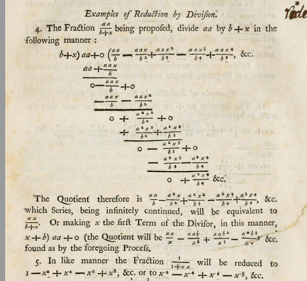


 ,
,