Calculus

A slant asymptote for a real function of one real variable $f$ is a line $y=ax+b$ with the property

$f(x)=ax+b+g(x)\qquad\qquad (1)$ ,

where $g(x)\to 0$ as $x\to\pm\infty$ . Geometrically, the graph of $f$ comes closer and closer to the line for large positive/negative values of $x$ . For the sake of simplicity, we will deal with asymptotes at $+\infty$ , the other case being completely analogous. When $a=0$ we say that the asymptote is horizontal. A simple way to detect if a given function has a slant asymptote is by checking linearity at infinity, ${\it i.e.}$ if the limit

$\displaystyle{\lim\limits_{x\to\infty}\frac{f(x)}{x}}$

is finite. If that is the case, the value of the limit is the slope of the asymptote, $a$ . The free term $b$ is then given by the limit

$\displaystyle{\lim\limits_{x\to\infty}f(x)-ax}$ ,

if the latter exists (and is finite). For rational functions of the form

$\displaystyle{f(x)=\frac{P(x)}{Q(x)}}$

where $P$ and $Q$ are polynomials, the situation is much simpler. In order for $f$ to be linear at infinity, we need ${\rm deg}(P)-{\rm deg}(Q)\le 1$ and, if that is the case, we perform long division which leads to

$\displaystyle{f(x)=ax+b+\frac{R(x)}{Q(x)}}\qquad\qquad (2)$

where ${\rm deg}(R)<{\rm deg}(Q)$ and, therefore, the asymptote is just the quotient $y=ax+b$ since

$\displaystyle{\lim\limits_{x\to\infty}\frac{R(x)}{Q(x)}=0}$

When ${\rm deg}(P)-{\rm deg}(Q)> 1$ , the fraction is superlinear at infinity.

All this is well known and usually taught in high school.

On the other hand, students are taught to find tangents to a given curve at a given point by means of derivatives. It turns out, however, that finding the tangent to a rational function at $x=0$ does not require derivatives at all. In order to understand this, we notice that $y=cx+d$ is a tangent to $f(x)$ at $x=0$ precisely when

$f(x)=cx+d+g(x)$

with $g(x)=o(x)$ as $x\to 0$ . The last relation is very similar to $(1)$ except for the fact that now we are looking at $x\to 0$ instead of $x\to\infty$ . Thus, if we could somehow come up with a relation like $(2)$ where now

$\displaystyle{\lim\limits_{x\to 0}\frac{R(x)}{xQ(x)}= 0}$ ,

the quotient would be the tangent.

As it happens, that is perfectly possible. All we need to do is divide the polynomials starting with the lowest powers (backwards), until we reach a “partial remainder” whose lowest degree is two or higher. Observe that the lowest degree of the divisor $Q$ is necessarily zero (otherwise $f$ is undefined at $x=0$ ).

As an example, let us find the tangent to the graph of

$\displaystyle{g(x)=\frac{2-2x+3x^2}{1+2x^2}}$

at $x=0$ . Starting with the lowest degree, we have $2=2\cdot 1$ , $2(1+2x^2)=2+4x^2$ with first partial remainder $R_1(x)=2-2x+3x^2-(2+4x^2)=-2x-x^2$ . In the next step, we add $-2x$ to the quotient, with a partial remainder $R_2(x)=-2x-x^2+2x(1+2x^2)=-x^2+4x^3$ . Since we are interested in the tangent line and $x^2$ is an infinitesimal of degree higher than one at zero, the division stops here and the equation of the tangent is $y=2-2x$ . If we keep dividing, we get the Taylor polynomials of higher degree. For instance, the osculating parabola at $x=0$ is $y=2-2x-x^2$ and so on.

Long division is taught at school starting with the highest powers. A possible reason is that long division of numbers proceeds by reducing the remainder at each step. If we replace the base $10$ in the decimal representation of numbers by $x$ , we arrive at the usual long division algorithms of polynomials, reducing the degree at each step. I would call this procedure “division at infinity”. In contrast, the above is an example of “division at zero”.

Finding the tangent to a rational function at a point different from zero can be reduced to the previous case. If, say, we need to find the tangent to $f(x)=P(x)/Q(x)$ at $x=x_0$ , all we need to do is set $x=x_0+z$ and express $P$ and $Q$ as polynomials in $z$ and then finding the tangent at $z=0$ as before. Finally, we have to replace $z$ back by $x-x_0$ in the found equation of the tangent.

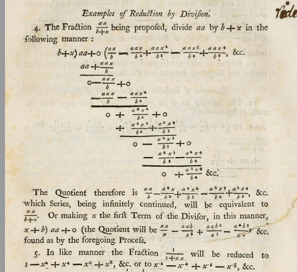
The above reveals a perfect symmetry between the problems of finding the asymptote and that of finding the tangent at $x=0$ . In some sense, we can say that an asymptote is a “tangent at infinity” and, I guess, that a tangent is an asymptote at a finite point. Both problems are algebraic in nature and can be solved without limit procedures, just by means of division (forward or backward).

More generally, for rational functions, being the simplest non-polynomial functions, finding their Taylor expansion at zero (and, by translation at any point) is a pure algebraic procedure. I believe this fact should be emphasized in high school and it could be used as a motivating example to introduce more general power expansions. As a matter of fact, Newton was inspired by the algorithm of long division for numbers to start experimenting with power series, not necessarily with integer powers. The image below shows a page from his “Method of Fluxions and Infinite Series”. The “backwards” long division of $a^2$ by $b+x$ is performed in order to get the power series expansion.

The differential of a quotient

Here is yet another example of “division at zero”.

When students are exposed to the differentiation rules, those are derived from the definition of derivative as the limit of the differential quotient. Thus for example to prove the rule of differentiation of a product we proceed as follows.

$\displaystyle{(fg)'(x)=\lim\limits_{h\to 0}\frac{(fg)(x+h)-(fg)(x)}{h}=}$

$\displaystyle{=\lim\limits_{h\to 0}\frac{f(x+h)g(x+h)-f(x)g(x)}{h}=\lim\limits_{h\to 0}\frac{f(x+h)g(x+h)-f(x+h)g(x)+f(x+h)g(x)-f(x)g(x)}{h}=}$

$\displaystyle{=\lim\limits_{h\to 0}f(x+h)\frac{g(x+h)-g(x)}{h}+\lim\limits_{h\to 0}g(x)\frac{f(x+h)-f(x)}{h}=}$

$\displaystyle{=f(x)g'(x)+f'(x)g(x)},$

given that all the limits are assumed to exist. A similar computation can be done for the quotient. It should be noted, however, that a little algebraic trick has to be used in both cases to make the derivatives of the individual factors appear explicitly. No big deal, but a bit artificial. And, importantly, not the way the founders of Infinitesimal Calculus arrived at these rules.

To help intuition, the product rule is often presented in the form

$d(uv)=(u+du)(v+dv)-uv=udv+vdu+dudv=udv+vdu$ ,

and the last term is ignored in the last equality as being a quadratic infinitesimal (in Leibniz’ terminology, the last equality is actually an “adequality”, a term coined by Fermat). Without a doubt, the latter derivation, albeit not meeting the modern standards of rigor, reveals the reason for the presence of the “mixed” terms and the general structure of the formula. Moreover, no algebraic tricks are required. The formula follows in a straightforward manner.

A similar derivation of the quotient rule involves “division at zero”. Here is the derivation in the book “Calculus made easy” by Silvanus Thompson, from 1910.

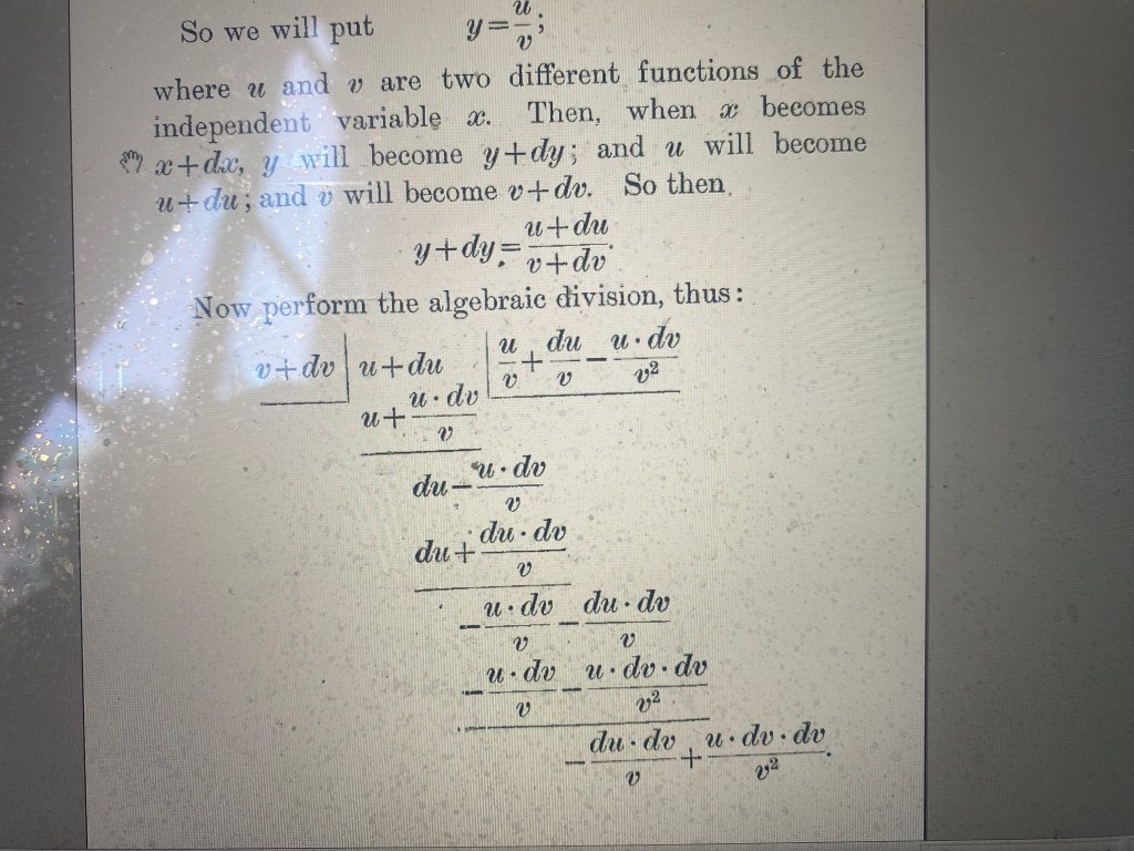
Observe that the operation has been stopped when the remainder is a quadratic infinitesimal. The conclusion of the computation is the familiar rule

$\displaystyle{d\left(\frac u{v}\right)=\frac{u+du}{v+dv}-\frac u{v}=\frac{du}v-\frac{udv}{v^2}=\frac{vdu-udv}{v^2}}.$

Math Bites

by Guillermo Reyes, PhD

Asymptotes, tangents and backwards long division

The differential of a quotient