The structure of the real line is deceptively intricate. Rational and irrational numbers are densely interwoven, yet they differ fundamentally—not just in their arithmetic properties, but in how they can be approximated. Even the rationals themselves possess a rich, hierarchical organization, elegantly captured by the Stern-Brocot tree.
If you take a course on Real Analysis where these matters are looked at in some detail, or an Algebra course where extensions of the rational field are considered (say, a course on Galois theory), you encounter the concepts of algebraic and transcendental numbers. Rational numbers can be thought as the ones solving a linear equation with integer coefficients, . A natural generalization leads us to the definition of algebraic numbers as real numbers satisfying a polynomial equation of the form with integer coefficients . The degree of an algebraic number is the lowest degree of a polynomial with integer coefficients having the given number as a root. Such polynomial has to be irreducible in , otherwise the said number would be a root of a lower degree polynomial. Real numbers which are not algebraic are called transcendental. Clearly, all rational numbers are algebraic, and all transcendental numbers are irrational.
The idea of the existence of transcendental numbers goes back to Leibniz, but the first to prove it, by giving a concrete example, was J. Liouville in papers from 1844 and 1851, [1] & [2]. It is often the case that when transcendental numbers are presented, the examples provided include , , and the Euler-Mascheroni constant or Apéry’s constant are mentioned as candidates (it is not even known if those are irrational). Proving that or are transcendental was accomplished by Hermite and Lindemann in the second half of the XIX century, and their proofs are far from elementary and can hardly be motivated and put in simple terms.
In contrast, Liouville’s constant has a very simple structure and the proof of its transcendency is completely elementary. It is defined as the number
,
that is, the number where the “ones” appear at positions given by the factorials, after the decimal point. Not being periodic, is clearly irrational.
Here is the reason why is transcendental: it can be approximated “too well” by the partial sums of the series, contradicting a result proved by Liouville, whose (very simple) proof is given below. The statement of the result, which we accept for the time being, is as follows.
Theorem [1] : Let be an irrational algebraic number of degree (i.e., is a root of an irreducible polynomial of degree with integer coefficients). Then there exists a constant such that for all rational numbers (with ) we have
.
(in words, algebraic numbers are not “too close” to rationals, in the sense that the rate of convergence of sequences of rationals with increasing denominators is limited by the degree of the given algebraic number). Formula should be contrasted with the well known fact that the continued fraction convergents of any irrational number satisfy
.
Liouville’s constant violates the theorem
The partial sums are rational numbers with denominator . It is clear that
On the other hand, if were algebraic of degree , we would have, according to Liouville’s Theorem,
But relations and clearly contradict each other for large . Indeed, for large enough , we have
,
since . Thus, is transcendental.
A proof of Liouville’s Theorem
Proof: By definition, there exists an irreducible polynomial in
with . If is a rational number in lowest terms (, then is a non-zero integer,
and therefore
.
Next, we relate to via the Mean Value Theorem,
for some between and . If we fix an interval around , that is, if we assume, say, , then and the previous estimate entails
.
The assertion follows with .
Final Remarks
During the time of Liouville and Hermite, transcendental numbers appeared rare and exotic, requiring ingenious proofs to isolate even a handful of examples. Yet just a few decades later, in 1874, Cantor demonstrated that, in fact, almost all real numbers are transcendental. What seemed like a hunt for “needles in a haystack” turned out to be a realization that the “haystack” was almost entirely made of “needles.” His proof, however, was non-constructive—relying not on explicit examples but on the abstract principles of cardinality and the countability of algebraic numbers.
Here is a question worth pondering: If almost all numbers are transcendental, why do the ones we encounter so rarely reflect that? Part of the answer to this question is probably that humans think algorithmically. We are drawn to numbers we can compute, describe, or construct. Most numbers are not describable.
The apparent simplicity of Liouville’s constant is deceptive—a trick of human intuition. What makes it seem simple is merely the ease of describing its decimal representation. By contrast, a number like might appear ‘chaotic’ in its decimal expansion, yet it is fundamentally structured: as a quadratic irrational, its continued fraction is perfectly periodic,
.
The same applies, for instance, to the golden ratio, again a quadratic irrational with a very simple continued fraction representation, etc. This reveals a deeper truth: our perception of mathematical simplicity often depends on the representation we choose, not the object itself.
I hope you enjoyed this dive into Liouville’s constant — its deceptively tidy decimal mask is, after all, a very human kind of charm.
[2] Liouville, J. (1851), “Sur des classes très étendues de quantités dont la valeur n’est ni algébrique, ni même réductible à des irrationnelles algébriques”, Journal de Mathématiques Pures et Appliquées, 16, 133–142. https://www.numdam.org/item/JMPA_1851_1_16__133_0.pdf
The Legendre transform has its origins in the work of A.M. Legendre [1], where it was introduced to recast a first order PDE into a more convenient form. It gained significance around 1830 with the reformulation of Lagrangian mechanics carried out by W. R. Hamilton by replacing the “natural” configuration space by the so called phase space with its rich symplectic structure [2] and as a central tool in Hamilton-Jacobi theory. In the late 19th century, it was used in Thermodynamics (Gibbs, Maxwell) as a way of switching between different thermodynamic potentials. With the development of Convex Analysis and Optimization in the 20th century, its central role in providing so called dual representations of functions, problems, etc. became apparent, [3].
From a high level point of view, the transform establishes a link between a function of a variable belonging to or a more general topological vector space and its “dual” or “conjugate” function, defined on the dual space of linear forms. From a more practical perspective, it can be understood as an alternative way of encoding the information contained in a function. In that sense, it is very similar to other transforms like the Fourier series/transform and the Laplace transform. The Fourier series, for instance, encodes the information about the given (periodic) function in the form of a sequence of “amplitudes” corresponding to the different “modes”. The Fourier transform furnishes a similar integral representation for non-periodic functions, where this time different “modes” or “frequencies” form a continuum. Both the series and the transform provide a spectral representation of the function.
Suppose we are given a convex real function of one real variable. Let us assume for simplicity that is twice differentiable and for all . Typical examples are quadratic functions with , exponential functions with , the function , etc.
Since , is a strictly increasing (hence one-to-one) function. Such correspondence allows to identify with the value of the slope of at that point, . In other words, can be used as a new independent variable. At this point, one might be tempted to use the function , where (or ) as an alternative representation of . This is, no doubt, a possible choice. However, a little extra work provides a function that has the following pleasant additional property: if the procedure is applied twice we recover the original function, . The transformation is what is called involutive (an involution).
Namely, given a slope , we start by identifying the point such that . You can think of this operation as parallel-transporting a line with slope in the direction of the axis starting from . Assuming that , there will be a first point of contact with the graph of . At this point, the graph is tangent to the line. We will encode this information by recording the point of intersection with the – axis; more precisely, if our line has equation , we define . The knowledge of the function is tantamount to the knowledge of all the tangents to our graph: our original graph is their (uniquely defined) envelope. The function is called the Legendre transform of . In the figure below, the values of the transform of the function at and are represented.
It is easy to derive an explicit formula for . Given , we need to solve for in the equation
The equation of the tangent is . Its -intercept is . Finally,
.
This new function is convex. Indeed, a simple computation shows that
.
From formula it follows that, given , we have
where, as before, . The formula above reveals that , (i.e. the transformation is involutive), since
There is another way to look at this. For fixed in the range of , the condition yields the (unique) critical point of the concave function . This point is a global maximum. Thus,
.
The latter equation implies the well-known Young’s inequality:
valid for any . Equality takes place when are linked by the relation .
Examples: If , . More generally, if with for , then , where . If , then , etc.
Generalizations
So far, we have assumed that our function is twice differentiable, with in its domain. However, the following slight modification of ,
is meaningful for any real and any function if we accept the values in the range of . The resulting function , being the supremum of a family of linear functions, is convex on its domain. Definition , however, is not completely satisfactory for non-convex functions, as it loses information about the original function. However, for a convex function defined on , encodes all the information about and, moreover, , a fact known as the Fenchel-Moreau theorem, [3]. Namely,
,
which can be thought as a representation of as the envelope of its tangents. For convex functions defined on some domain , an extra technical condition is needed on for to hold, namely lower semicontinuity, which is equivalent to the closedness of its epigraph. It is easy to see that this is a necessary condition for to hold. Indeed, furnishes a representation of the epigraph of as an intersection of closed half-planes, hence necessarily closed.
In the context of Convex Analysis, the more general transformation given by is called the Fenchel transform (or Fenchel-Legendre transform) and the more general inequality is called the Fenchel inequality (or Fenchel-Young inequality).
Thus, the transformation can be applied to a piece-wise linear, convex function. For instance, if is a linear function, , then clearly is finite only for , with . If is made of two linear functions, when and when , with and , then is finite only for , where it is linear and ranges from to . In general, to each “corner” of a polygonal graph there corresponds a segment on the graph of , [2].
The generalization to functions is straightforward. Under the smoothness and strict convexity assumption
,
the mapping is one-to-one. If is the vector representing via the standard Euclidean structure, we define the Legendre transform by
,
where denotes the inner product. Much like in the one-dimensional case, the previous definition is equivalent to
.
Finally, we relax the smoothness and strict convexity assumptions and arrive at the most general definition
,
where now is merely convex and . The Fenchel-Moreau theorem holds without modifications under the extra assumption of lower semicontinuity of if it is not defined on all of .
One can also consider “partial” Legendre transforms, i.e. transforms relative to some of the variables. Thus if is a function of two variables, one can consider its transform with respect to the first variable,
.
For smooth, strictly convex functions and fixed , the supremum is achieved at the (unique) defined by
.
The transform can be further generalized to functions on manifolds, but given the fact that a manifold does not have a global linear structure, the duality is established locally, between functions on the tangent bundle and their “conjugates” or “dual” on the cotangent bundle . Namely, the transform connects functions of with functions of , where and .
Applications
A)Clairaut’s differential equation
A standard example of ODE not solved for the derivative is Clairaut’s equation
.
It clearly admits the family of straight lines as solutions. The envelope of the family is a singular solution satisfying and . But these are precisely the relations defining the Legendre transform of . We conclude that, for convex , the singular solution of Clairaut equation is its Legendre transform.
B)Hamiltonian Mechanics from Lagrangian Mechanics.
For many Physics, Applied Math, and Engineering students, this is their first introduction to the Legendre transform. The Lagrangian of a mechanical system on its configuration space (a differentiable, Riemannian manifold) completely describes the system. The actual path joining two states and is an extremal of the action functional,
(Hamilton’s principle) and therefore satisfies Euler-Lagrange second order differential equations
.
Te geometry of the configuration space is intimately connected to the Physics. Thus, holonomic constraints are built into the manifold, the kinetic energy is nothing but the Riemannian metric on the manifold, geodesics relative to this metric represent motion “by inertia”, etc. The alternative Hamiltonian description reveals connections to a different geometry and is introduced as follows. Assuming that the Lagrangian is strictly convex in the generalized velocities ,
we introduce the Hamiltonian of the system as the Legendre transform of the Lagrangian with respect to :
,
where is the generalized momentum, an element of the cotangent fiber at . Since
it follows that satisfy the first order Hamiltonian system:
The space is called the phase space, and the Hamiltonian function equips it with a remarkable symplectic structure. The Hamiltonian flow (if does not depend on time) is a one-parameter subgroup of the group of symplectomorphisms of the phase space. A straightforward consequence is Liouville’s Theorem on the preservation of the phase volume (a cornerstone of Statistical Mechanics) . The Lagrangian approach has, however, certain advantages including: a) it is easier to deal with constraints, even non-holonomic via Lagrange multipliers; b) it is easier to track conserved quantities via Noether’s theorem, c) non-conservative forces can be incorporated, etc.
It is worth noticing that the above “Hamiltonization” applies to general variational problems, not just to the problem related to mechanical systems. In the case of mechanical systems, the part of the Lagrangian depending on is usually a positive definite quadratic function (the kinetic energy of the system) hence convex. The transform of a quadratic form is especially simple: it is just another quadratic form of the conjugate variable. For instance, the Lagrangian of a simple mass-spring system, assuming that the spring is linear and represents the deviation of the mass from equilibrium is
and the Hamiltonian is
and represents the total energy of the system. That is the case whenever the Lagrangian is quadratic on velocities, the system is conservative and the constraints are time-independent.
C)Thermodynamic potentials
Yet another early use of the transform was in Thermodynamics, as a way to switch between potentials according to the most convenient independent parameters.
According to the first principle of Thermodynamics (energy conservation), there exists a function of state (internal energy) such that, for any thermodynamical system undergoing an infinitesimal change of state,
,
where represent the heat (thermal energy) added to the system, is the work of the surroundings on the system and the last sum above accounts for the energy added to the system by means of particle exchange. Here, is the amount of particles of the -th type added to the system, and the corresponding chemical potential. The relevant fact here is that is an actual differential, whereas the rest of the terms are just differential forms in the configuration space of the system. The term is in general a differential form involving intensive () and conjugate extensive variables . Thus, for example, in the case of a gas expanding/compressing against the environment, the work done on the gas is , where is the infinitesimal change of volume and is the external pressure. Moreover, according to the second principle, for reversible processes the form admits an integrating factor , namely there is a function of state called entropy such that
Putting all together, for an infinitesimal, reversible (hence quasi-static) process undergone by a gas we get
where is the pressure of the gas in equilibrium with its surroundings.
While accounts for the total energy of the system, related state functions accounting for different manifestations of energy may result more convenient for particular experimental or theoretical scenarios. For instance, many chemical reactions occur at constant pressure in lab conditions. In such cases, it is convenient to include a term representing the work needed to push aside the surroundings to occupy volume at pressure , namely we define the enthalpy of the system as
.
Given that, thanks to we have , is nothing but (minus) the Legendre transform of with respect to , that is,
.
(in Thermodynamics, the transform is usually defined with opposite sign so there is no “minus” in the previous formula. A possible reason is that one prefers all forms of energy to increase/decrease in agreement). Assuming for simplicity that we have
and, therefore, at constant pressure, . Thus, the change of enthalpy determines if a given chemical reaction is exothermic or endothermic. Moreover, and .
In a similar fashion, one can consider the (opposite of) Legendre transform of with respect to entropy,
,
called (Helmholtz) free energy. A similar computation shows that
,
thus we can think of as the pressure-volume work on the system under fixed temperature.
Yet another thermodynamic potential, the Gibbs free energy, is a measure of the maximum reversible work a system can perform at constant pressure (P) and temperature (T), excluding expansion work. It is useful to determine if a given process occurs spontaneously (e.g., chemical reactions, phase transitions) and equilibrium conditions.
Bibliography
[1] Legendre, A. M., “Mémoire sur l’intégration de quelques équations aux différences partielles.”Histoire de l’Académie Royale des Sciences, 1789, pp. 309–351.
[2] Arnold, V. I. “Mathematical Methods of Classical Mechanics”, 2nd Edition, Graduate Texts in Mathematics (60), 1989.
[3] Boyd, Stephen P. and Vandenberghe, L. “Convex Optimization“. Cambridge University Press, 2004.
Fig.1. (L) The Lipschitz condition for a function . (R) Rudolph Lipschitz (1832 -1903)
A classic condition on the right hand side of a first order normal ODE
guaranteeing local uniqueness of solutions with given initial value is Lipschitz continuity of in the variable in some open, connected neighborhood of where is defined. That is, it is required that there exist some constant such that
for all in . Under the above condition there is a unique local solution of the initial value problem
where uniqueness means that two prospective solutions defined on open intervals containing coincide in their intersection. We assume that our solutions are classical, , continuously differentiable. Such solutions exist when extra conditions on are imposed. For instance, if is assumed continuous in , classical local solutions exist and can be extended up to the boundary of . But here our concern is uniqueness.
My goal here is to explain why such condition implies uniqueness in simple terms, how it can be generalized and the relation between uniqueness and another interesting phenomenon, namely finite-time blow-up of solutions.
To illustrate the idea, we will assume that and . We will also assume that for every and, therefore, one solution of the above IVP is . The general case reduces to this one, as we explain later.
We focus on forward uniqueness. Namely, we will prove that a solution with for some can never be zero at . We will assume , as the case can be handled in a similar way. Backwards uniqueness also follows easily from the forward result.
Uniqueness is violated if, as decreases from to zero, vanishes at some point , , while for . By the Lipschitz condition,
while . It then follows from the ODE that
along the solution for . Integrating this inequality over ,
This integral inequality is the crux of the argument. Just observe that, since the improper integral is divergent, approaching zero would require , contradicting the assumption as . The Lipschitz condition prevents from becoming zero over finite -intervals.
The argument above is equivalent to the following: for any solution with for some one can construct an exponential barrier from below of the form for some , that is, for all in its domain, thus preventing from becoming zero. Indeed, the inequality
implies that our solution is increasing at a slower pace than the solution of the IVP
which is nothing but for the appropriate . Therefore, to the left of . In other words, acts as a lower barrier for , as in the figure below.
Fig 2. The exponential barrier prevents the solution through from reaching the -axis.
If we assume that , we use the inequality (again a consequence of )
for to conclude that with is a barrier from above for our solution, preventing it from reaching the -axis.
The integral inequality suggests a very natural generalization. Indeed, all we need is a diverging (at zero) improper integral on the right-hand side. We can replace the Lipschitz condition by the existence of a modulus of continuity, that is a continuous function with , for satisfying
in , with the additional property
.
This more general statement is due to W. Osgood. The Lipschitz condition corresponds to the choice . The proof is identical to the one above, given that the only property we need is the divergence of the improper integral of at .
Thus, for an alternative solution to branch out from the trivial one, we require a non-Lipschitz right-hand side in that leads to a convergent improper integral. This condition is satisfied, for instance, in the autonomous problem
which, apart from the trivial solution, has solutions of the form on and for for any .
There is nothing special about the power in this example. Any power with would do. These examples of non-uniqueness are usually attributed to G. Peano.
Uniqueness for general solutions can be easily reduced to the special case above. Namely, if and are local solutions of (say on ), then is a local solution of
on with . Moreover, satisfies a Lipschitz condition near if does near , with the same constant . By the above particular result, and hence on the corresponding intervals.
Remarks: A simple and widely used sufficient condition for to hold is the continuity of the partial derivative in an -convex region (typically a rectangle). This follows from a straightforward application of Lagrange’s mean value theorem; is not necessary for uniqueness, as the example of with with shows; The Lipschitz condition is relevant in other areas of Analysis. For instance, it guarantees the uniform convergence of Fourier series.
A related phenomenon: blow up in finite time.
Local solutions issued from can be extended to the boundary of , but not necessarily in the -direction. The reason is a fast (superlinear) grow of as , assuming that the domain of definition of extends indefinitely in the -direction. A simple example is the problem
,
whose explicit solution “blows up” as , despite the fact that is smooth on the whole plane. The role of the superlinear growth at infinity is similar to the role of Lipschitz (or Osgood) condition in bounded regions for uniqueness. The above problem is equivalent to
Convergence of the improper integral prevents from attaining arbitrarily large values. Calling , we have . This phenomenon is called finite time blow-up and is exhibited by ODEs with superlinear right-hand-sides, by some evolution PDEs with superlinear sources, etc.
The same reasoning applies in the general case when there exists a continuous such that as (resp. as ) if only
.
This time, under assumptions guaranteeing existence and uniqueness of solutions and provided the first condition above holds, the (forward) solution to with stays to the left of the solution of
with . The latter blows up in finite time, namely at time , forcing the solution to our IVP to blow up at some .
Main contributors to the theory of real numbers. From left to right: Eudoxus, S. Stevin, G. Cantor and R.Dedekind.
Nowadays students are exposed to the concept of “real line” as a model of the one-dimensional continuum in middle school. The real line contains all previously encountered classes of numbers: natural, integers, rational and irrational and no “gaps” are left. This object, so ubiquitous in modern mathematics, constitutes the basis upon which all of Calculus, Real and Complex Analysis and Linear Algebra (over or ) are built.
It may come as a surprise the fact that the concept crystallized relatively recently, after a slow and painful evolution of the concept of number over the centuries, with contributions from various civilizations shaping our current understanding.
In the Western hemisphere, as far as a systematic development is concerned, the story starts in ancient Greece around 500 BC. Greeks derived their Mathematics from older Egyptian and Babylonian traditions, which viewed Mathematics as a practical tool for counting and measuring.
According to Plato (Philebus 56D-57E, see [2]), there were two kinds of Mathematics in Greece, “that of the people and that of philosophers”. The mathematics of the people was called logistics (λογιστική) and followed the Egyptian/Babylonian tradition. It was concerned with calculations and measurement. That of philosophers, especially appreciated by Plato (429-348 BC) was viewed as a means for apprehending truth. Accordingly, they had a nuanced understanding of numbers. Only counting or natural numbers except for the number one were “numbers” in their own right for them. They used the term “arithmos” (ἀριθµός) for those numbers, and “arithmetic” (ἀριθμητική) for the related study. The reason why the unit was not considered a number was rather philosophical: the unit was a monad, related to the “essence” and indivisible, while a number, by definition, is a multitude of units. This ontological distinction is made by Aristotle in his Metaphysics, 1039a15 and elsewhere, and it is the historical reason why “one” was not considered a prime number. It was not a number at all!
Here is another nuance of Greek mathematics: they would carefully distinguish between numbers and magnitudes. Those belonged to completely different realms. Numbers were discrete whereas magnitudes were continuous. There were different kinds of magnitudes: lengths, areas, volumes, times, etc. When Greeks referred to a magnitude, they did not have a number in mind. A length was a portion of a line; an area was a portion of the plane. Their formulation of Pythagorean Theorem, for instance, involved squares built on the legs and the hypothenuse of a right triangle, and the proofs amounted to shape rearrangements.
Apart from “arithmos”, Greeks had the concept of “logos” (λόγος), which can be translated as “ratio”. These “fractions” were not actual numbers and served the purpose of attaching a “relative” size to magnitudes. According to Elements, Book V, Definitions 3 and 4, “a ratio is a sort of relation in respect of sizebetween two magnitudes of the same kind”. However, it did not make sense for them to consider the ratio of a length to an area, or of length to time (mixed ratios). They only considered ratios of magnitudes of the same kind and ratios of numbers. Ratios could be compared between magnitudes of different kinds by means of proportions. Here is an example, [2]: “Triangles and parallelograms which are under the same height are to one another as their bases” (Elements, book VI).
Numbers can be added and subtracted, and so can magnitudes of the same kind, but ratios cannot. An abstract interpretation of the concept of ratio in Greek mathematics can be found in Bourbaki, [3]: “the ratios of integers are conceived by the classical Greek mathematicians as operators, defined on the set of integers or on a part of this set (the ratio of p to q is the operator which, to , makes correspond, if is a multiple of , the integer , a multiple of “.
Discovery of Incommensurability
A significant milestone in Greek mathematics was the discovery of incommensurability, traditionally attributed to the Pythagoreans. They found that some lengths, such as the diagonal of a square and its side, could not be “measured with a common unit”. In other words, there were not enough ratios of numbers to account for all possible ratios of magnitudes. According to Fowler [2], the discovery may be related to experimentation with anthyphairesis (the Euclidean algorithm/continued fractions) by noticing that in some cases the process continued indefinitely, and no common unit could be thus found. Anthyphairesis applied to the side and the diagonal of a square or to the side and the diagonal of a pentagon easily lead to a periodic continuous fraction and consequent incommensurability. Thus for example, the ratio of the diagonal of a square to its side (which we identify with the real number ) produces the continuous fraction
.
In many modern textbooks it is claimed that the Pythagoreans discovered that the number was irrational. Such claim is anachronistic and inaccurate; neither fractions or were numbers at all.
Eudoxus’ Theory of Proportions
In response to the problem of incommensurability, Eudoxus, who lived in the third century BC and attended Plato’s Academy, developed the so called theory of proportions. Eudoxus’ theory, as rendered in Euclid’s Elements, provided a way to compare (homogeneous) magnitudes, narrowing the gap between arithmetic and geometry. Namely, “magnitudes are said to be in the same ratio, the first to the second and the third to the fourth, when, if any equimultiples whatever be taken of the first and third, and any equimultiples whatever of the second and fourth, the former equimultiples alike exceed, are alike equal to, or alike fall short of, the latter equimultiples respectively taken in corresponding order. When, of the equimultiples, the multiple of the first magnitude exceeds the multiple of the second, but the multiple of the third does not exceed the multiple of the fourth, then the first is said to have a greater ratio to the second than the third has to the fourth” (Elements, Book V, Def. 5). In other words, given four magnitudes we say that the first is to the second as the third is to the fourth, if, for any integers the following equivalencies hold
,
and similarly for the “less than” and the “greater than” relations between ratios. If two magnitudes and are commensurable, there exist integers and such that the equality relation above holds. If they are incommensurable, the two extreme relations furnish “rational approximations” to the given ratio . But again, neither those rational approximations or the final ratio were “numbers”.
The main advantage of Eudoxus’ theory was that it could be applied to both commensurable and incommensurable magnitudes, see Heath [1]. It foreshadows the construction of real numbers given by Dedekind over two millennia later.
Such was the official position of Greek mathematics, as portrayed in their most influential text, the Elements of Euclid, around 300 BC.
Logisticians, on the other hand, viewed fractions as numbers and freely added and subtracted them, specially fractions with numerator equal to one, following the Egyptian tradition.
The Hellenistic Period and Beyond
During the Hellenistic period, Greek Mathematics continued to build on the above concepts. Archimedes made significant contributions to the understanding of numbers and geometry, including the approximation of using the method of exhaustion that had been introduced by Eudoxus and related to the above rational approximations of the perimeter/radius ratio. Notably, Archimedes applied this method to the computation of areas of non-trivial shapes (parabolic sector, sector bounded by an arc of a spiral, etc.) Many applications of this method can be found in the Book XII of the Elements.
With the decline of Greek Mathematics in the third century AD, philosophical considerations gave way to a return of the naiver point of view of logisticians, [3]. A representative of that period is Diophantus of Alexandria, who was the first mathematician to recognize (positive) fractions as numbers. His main motivation came from Algebra, by accepting rational and even irrational numbers as possible values for coefficients and solutions to algebraic equations. Arithmetica is the major work of Diophantus and the most prominent work on premodern Algebra in Greek mathematics. Thus, a major advancement, namely the development of Algebra, was accompanied by a conceptual regress, [3].
Medieval Developments and Stevin’s Innovations
The medieval period saw a relative stagnation in the advancement of Mathematics in Europe, but significant progress was made in the Islamic world. Mathematicians like Al-Khwarizmi and Omar Khayyam expanded on Greek ideas and introduced algebraic methods that would later influence European mathematics. Among other things, negative numbers were introduced about 620 CE in the work of Brahmagupta (598 – 670) who used the ideas of ‘fortunes’ and ‘debts’ for positive and negative. By this time a system based on place-value was established in India, with zero being used in the Indian number system.
The Renaissance brought a resurgence of interest in mathematics in Europe. Arithmetica was first translated (never published) from Greek into Latin by R. Bombelli in 1570. Bombelli realized that, once a unit of length is chosen, there is a one-to-one correspondence between ratios and lengths. He thus had a geometric version of the real numbers. In his Algebra, he was the first European who clearly stated (and gave geometric proofs of) the rules for multiplication of positive and negative numbers: , etc. Bombelli is also responsible for an early use of “imaginary” numbers for the solution of cubic equations.
In the same century, Simon Stevin, a Flemish mathematician, adopting the point of view of Bombelli, made groundbreaking contributions by advocating for the use of decimal fractions. In his work De Thiende (The Tenth, published in 1585), Stevin demonstrated how fractions could be represented as decimal numbers, making calculations more straightforward and paving the way for the inclusion of irrational numbers in arithmetic. For the first time, the unit, fractions and irrational numbers were members of one and the same numerical field. In Stevin’s own words: “We conclude therefore that there are no absurd, irrational, irregular, inexplicable or deaf numbers; but that there is in them such excellence and agreement that we have subject matter for meditation night and day intheir admirable perfection”.
Stevin’s work was crucial in transitioning from a purely geometric interpretation of numbers to a more algebraic and analytical approach. His decimal fractions also inspired Newton’s study of infinite series.
The real line
The first mention of the number line used for operation purposes is found in John Wallis’s (1616 – 1703) Treatise of Algebra. In his treatise, Wallis describes addition and subtraction on a number line in terms of moving forward and backward, under the metaphor of a person walking. The one-to-one correspondence between points on a line and numbers had been established.
René Descartes (1596 – 1650) took the idea further with his introduction of the Cartesian coordinate system on the plane and in space. In his work La Géométrie Descartes linked Algebra and Geometry, allowing geometric problems to be solved algebraically and viceversa. This unification laid the foundation for Analytic Geometry. The analytic study of curves gave rise to the birth of Calculus. The introduction of coordinates is essential to the construction of many physico-mathematical theories like Mechanics, Electromagnetic Theory, Thermodynamics, Statistical Mechanics, &c.
A rigorous construction
Stevin’s decimals did not lend themselves to a satisfactory construction of real numbers, in particular they did not provide sound definitions of the operations of sum and multiplication. The year 1872 saw the publication of work by G. Cantor and R. Dedekind, who independently provided a rigorous construction of real numbers out of rationals. Cantor’s construction is based on classes of equivalency of “Cauchy sequences” of rational numbers, whereas Dedekind’s approach hinges on the concept of “cut”, and is conceptually very close to Eudoxus’ theory of proportions. Both constructions were possible thanks to the recently developed language of the theory of sets, which allowed to consider sets of very large “size” (more precisely, cardinality). Such flexibility raised suspicion from many relevant scholars and a decades long debate ensued. Although the construction of reals by Cantor and Dedekind have been largely accepted and is regularly taught at colleges and universities, alternative schools of thought including Intuitionism and Finitism are still in existence and have developed their own Mathematics based on restricted versions of Set Theory, restricted Logic, etc.
Beyond the reals
We should also mention that alternative constructions of the continuum, built upon standard Set Theory, have been proposed starting in the last decade of the XIXth century. A full reconstruction of Analysis was proposed in the 1960s by A. Robinson, culminating with his Nonstandard Analysis, published in 1966. In his work, the real line is replaced by a non-Archimedean”hyperreal” one, containing actual infinitesimals and infinities of different orders along with ordinary real numbers. The main goal was to remove the concept of limit and construct a purely “algebraic” version of Analysis, thus vindicating the dream of Leibniz. But this is a major and intricate topic that deserves a separate post.
References
[1] Sir T. Heath, “A History of Greek Mathematics”, Oxford Clarendon Press, 1921.
[2] D.H. Fowler, “Ratio in Early Greek Mathematics”, Bulletin of the AMS, Vol 1 (6), 1979.
[3] N. Bourbaki, “Elements of the History of Mathematics”, Springer, 1999.
A slant asymptote for a real function of one real variable is a line with the property
,
where as . Geometrically, the graph of comes closer and closer to the line for large positive/negative values of . For the sake of simplicity, we will deal with asymptotes at , the other case being completely analogous. When we say that the asymptote is horizontal. A simple way to detect if a given function has a slant asymptote is by checking linearity at infinity, if the limit
is finite. If that is the case, the value of the limit is the slope of the asymptote, . The free term is then given by the limit
,
if the latter exists (and is finite). For rational functions of the form
where and are polynomials, the situation is much simpler. In order for to be linear at infinity, we need and, if that is the case, we perform long division which leads to
where and, therefore, the asymptote is just the quotient since
When , the fraction is superlinear at infinity.
All this is well known and usually taught in high school.
On the other hand, students are taught to find tangents to a given curve at a given point by means of derivatives. It turns out, however, that finding the tangent to a rational function at does not require derivatives at all. In order to understand this, we notice that is a tangent to at precisely when
with as . The last relation is very similar to except for the fact that now we are looking at instead of . Thus, if we could somehow come up with a relation like where now
,
the quotient would be the tangent.
As it happens, that is perfectly possible. All we need to do is divide the polynomials starting with the lowest powers (backwards), until we reach a “partial remainder” whose lowest degree is two or higher. Observe that the lowest degree of the divisor is necessarily zero (otherwise is undefined at ).
As an example, let us find the tangent to the graph of
at . Starting with the lowest degree, we have , with first partial remainder . In the next step, we add to the quotient, with a partial remainder . Since we are interested in the tangent line and is an infinitesimal of degree higher than one at zero, the division stops here and the equation of the tangent is . If we keep dividing, we get the Taylor polynomials of higher degree. For instance, the osculating parabola at is and so on.
Long division is taught at school starting with the highest powers. A possible reason is that long division of numbers proceeds by reducing the remainder at each step. If we replace the base in the decimal representation of numbers by , we arrive at the usual long division algorithms of polynomials, reducing the degree at each step. I would call this procedure “division at infinity”. In contrast, the above is an example of “division at zero”.
Finding the tangent to a rational function at a point different from zero can be reduced to the previous case. If, say, we need to find the tangent to at , all we need to do is set and express and as polynomials in and then finding the tangent at as before. Finally, we have to replace back by in the found equation of the tangent.
The above reveals a perfect symmetry between the problems of finding the asymptote and that of finding the tangent at . In some sense, we can say that an asymptote is a “tangent at infinity” and, I guess, that a tangent is an asymptote at a finite point. Both problems are algebraic in nature and can be solved without limit procedures, just by means of division (forward or backward).
More generally, for rational functions, being the simplest non-polynomial functions, finding their Taylor expansion at zero (and, by translation at any point) is a pure algebraic procedure. I believe this fact should be emphasized in high school and it could be used as a motivating example to introduce more general power expansions. As a matter of fact, Newton was inspired by the algorithm of long division for numbers to start experimenting with power series, not necessarily with integer powers. The image below shows a page from his “Method of Fluxions and Infinite Series”. The “backwards” long division of by is performed in order to get the power series expansion.
The differential of a quotient
Here is yet another example of “division at zero”.
When students are exposed to the differentiation rules, those are derived from the definition of derivative as the limit of the differential quotient. Thus for example to prove the rule of differentiation of a product we proceed as follows.
given that all the limits are assumed to exist. A similar computation can be done for the quotient. It should be noted, however, that a little algebraic trick has to be used in both cases to make the derivatives of the individual factors appear explicitly. No big deal, but a bit artificial. And, importantly, not the way the founders of Infinitesimal Calculus arrived at these rules.
To help intuition, the product rule is often presented in the form
,
and the last term is ignored in the last equality as being a quadratic infinitesimal (in Leibniz’ terminology, the last equality is actually an “adequality”, a term coined by Fermat). Without a doubt, the latter derivation, albeit not meeting the modern standards of rigor, reveals the reason for the presence of the “mixed” terms and the general structure of the formula. Moreover, no algebraic tricks are required. The formula follows in a straightforward manner.
A similar derivation of the quotient rule involves “division at zero”. Here is the derivation in the book “Calculus made easy” by Silvanus Thompson, from 1910.
Observe that the operation has been stopped when the remainder is a quadratic infinitesimal. The conclusion of the computation is the familiar rule
In pre-epsilontic times, mathematicians understood definite integrals as continuous sums of infinitesimals (in the above image, a page from Leibniz where he introduces the signs for difference and for sums. He uses the sign for adequalities). In the hands of the Bernoullis, Huygens, Euler, Lagrange, Legendre and many others, Infinitesimal Calculus, including the theory of differential equations as well as numerous applications to Mechanics, Optics, etc. developed for over 150 years under that conceptual framework. The situation changed during the second half of the XIX century, when set theory and a rigorous construction of the continuum was put forward by Cantor and Dedekind. Supposedly, they provided a final answer to the nature of the continuum that has been prevalent for over 150 years by now. Such a sparse ontology did not convince everyone, and there have been numerous alternative models of the continuum developed over time, aimed at restoring the language of infinitesimals, see [1]. As for the concepts of derivative and integral, infinitesimal interpretations were replaced by epsilons and deltas at the hands of Bolzano, Cauchy and, notably, Weierstrass.
Let us recall the definitions for the sake of completeness. For a real function of a real variable , if is a point in the closure of , we say that if for any there exists some such that
Both derivatives and integrals are limits. The derivative of at a point in the interior of is the limit
whenever the latter is finite. In the case of the definite integral over , we consider partitions , where with tags and form the Riemann sums
.
If the above sums have a finite limit as (uniformly w.r.t. the partitions and the tags), we say that is Riemann-integrable with integral equal to . Back to the language of epsilons and deltas, we are requiring that for any there exists such that
I am not concerned here with the alternative constructions of the continuum and the non-standard approach. My main concern is the teaching of (standard) Calculus. It is my belief that the main difficulties encountered by students when faced with the above definitions are philosophical/psychological in nature, as they feel a disconnection with good old Algebra and finite procedures. In order to fill the gap, I believe that the language of infinitesimals is to be preferred, specially in introductory courses. As I pointed out elsewhere, this is the language used by most users of Calculus, including Physicists and Engineers. Just like derivatives are quotients of infinitesimals, integrals are sums of infinitesimals, thus revealing a common theme. In other words, I believe that Calculus should be presented as an algebra of infinitesimals.
The main objection to this approach is the fact that infinitesimals cannot be properly defined in the realm of standard Calculus, based on the standard real line. I believe however that the pedagogical advantages stemming from its more intuitive character and its agreement with the historical evolution of the subject is worth the lack of rigor on a first acquaintance with the subject.
Let’s consider the different types of sums used in Calculus.
Adding two numbers is an operation everyone is familiar with. The (inductive) extension to a finite amount of addends is trivial, thanks to associativity. Here we are in the realm of Algebra.
Things become trickier when we intend to add infinitely many numbers. We already encounter this situation In Zeno’s paradoxes: In order to travel a certain distance, say , one has to travel half of the distance, then a fourth of the distance, then an eight of it, etc. Zeno rejected the possibility of such process made of infinitely many steps since, in his opinion, it could never be completed. Thus for Zeno and the followers of Parmenides, motion did not exist. Greek mathematics rejected completed infinite processes in general (see [2]) and therefore could not attach a numerical value to the “infinite sum”
Standard modern mathematics, however, has embraced the idea of the continuum through the concept of real number, originated with Simon Stevin and his decimal representations. Thanks to a hypostatic abstraction, now we declare numbers (real numbers) a certain property of sequences of rational numbers. In simpler terms, we adjoin to the number system all potential “limits”. Such construction would have abhorred Eudoxus and Euclid, but Cantor and Dedekind, along with most current mathematicians, were perfectly comfortable with it. In order to circumvent Zeno’s paradox, we start by defining the concept of infinite sum. The simplest choice, as is well known, is to consider “partial sums”
which in this case can be easily computed in closed form, , and then noticing that “stabilizes towards “, and thus has the real number as its limit, according to the standard paradigm. In modern terminology, we would say that we are dealing with a convergent series, whose sum is .
Several comments are in order. we are free to choose what we mean by an infinite sum, as the concept cannot be reduced to that of a finite sum. There are other choices (Cesaro’s convergence, for example) ; this mathematical construction does not solve the paradox, which belongs in the realm of metaphysics; in this example, the sum happens to be a rational number, but the concept of real number allows to attach a sum to series like
which is the “irrational” number .
A necessary condition for the series to have a finite sum in the above sense is that the general term of the sequence converge to zero, . Indeed, if stabilizes, the difference has to vanish asymptotically. The elementary theory of numerical series shows that this condition is not sufficient and that there are two main mechanisms of convergence: the general term converges to zero fast enough and the series contains infinitely many positive and negative terms and cancellations occur.
As an example of the first mechanism, any series of geometrically decreasing terms like the one above is convergent. Also, any series whose terms behave asymptotically as those of a convergent geometric series is convergent (this is called the ratio test). A relevant example of cancellation is given by Leibniz’s series above, where the partial sums oscillate around .
Summing up, for a sum over a discrete set of indices to be finite, the terms have to become small in a way that balances the number of addends, stabilizing the partial sums towards a finite limit.
Definite integrals showcase the next level of summation. In Riemann’s construction with uniform partitions, generic terms of the Riemann sums are of the order of , thus balancing the number of addends . In contrast with series, in this case the terms become arbitrarily small simultaneously, allowing for a “larger” number of addends, namely the continuous sum
over the set of indices . We can think of as the infinitesimal addends making up the sum. The situation here is more delicate, since all the terms making up the Riemann sums change every time and the values of the sums may not stabilize if the function is too discontinuous. Everything works nicely for continuous functions though.
When a Physicist needs to find the total mass of a non-homogeneous bar with density , he/she reasons as follows: choose an infinitesimal portion of the bar of length between two infinitesimally close points and . Being infinitesimal, the density is constant and equal to on that portion and the corresponding mass is . The total mass is thus the sum of the infinitesimal masses
.
Physics and Engineering books contain plenty of such formulas to compute extensive magnitudes. Yet the way Calculus is currently taught is at odds with the above line of thought. A colleague engineer once told me “I had to relearn Calculus. The version mathematicians taught me was useless”.
The balance between the cardinality of the set of indices and the size of the terms is critical. For instance, if we consider “Riemann sums” of either form
the corresponding limits are trivial,
for “reasonable” (say, continuous on ) functions. Indeed, in the first case the addends are too small, while they are too big in the second one: as .
We can further consider sums over a doubly continuous set of indices . Those are double integrals
,
where the addends are quadratic infinitesimals with respect to and . The same applies to general multiple integrals. Unbalanced Riemann sums give rise to trivial objects like
,
etc.
I believe formulas like provide deeper insight than all the technicalities related to the definition of the definite integral. They help understand why the concept of definite integral is relevant as it strikes the sweet spot where the “number of addends” (i.e. the cardinality of the set of indices) and their size balance each other, resulting in convergence to a finite, nontrivial sum.
References:
[1] “Ten misconceptions from the history of Analysis and their debunking”, P. Blaszczyk, M.G. Katz and D. Sherry, https://arxiv.org/pdf/1202.4153.pdf
[2] “Elements of the history of Mathematics”, N. Bourbaki, Springer Science & Business Media, 1998.
Sets of points satisfying certain geometric condition are ubiquitous in Mathematics. The simplest examples are straight lines, circles and more general conics. Thus a straight line can be defined as the set of points equidistant from two given points, a circle as the set of points whose distance to a fixed point (center) is constant and a conic as the set of points such that the ratio of the distances to a given point (focus) and a given line (directrix) is constant. The type of conic depends on whether the ratio (called eccentricity) is less, equal or greater than one.
Straight lines and circles were intensively studied since antiquity. They were the favorite objects of Greek geometers, and their properties are thoroughly investigated in Euclid’s Elements. In his fundamental treatise “Conics”, Apollonius of Perga, known as the “Great Geometer”, went further, tackling a systematic study of conics, establishing their focal properties, as well as those of chords and tangents, “conjugate” diameters, asymptotes, etc. It is believed that he heavily drew from previous work by Euclid as well as from Menaechmus, who is generally considered the discoverer of conic sections.
Greeks did not stop there. For the purpose of solving construction problems not amenable to the straightedge and the compass, they introduced more sophisticated loci like conchoids and cissoids, and “kinematic” curves like the quadratrix or the Archimedean spiral.
When the method of coordinates was introduced by Fermat and Decartes in the XVII century, the sophisticated auxiliary constructions typical of synthetic geometry were replaced by more straightforward and systematic algebraic methods. The equations of the above mentioned curves were obtained right away by expressing their defining properties in the language of Algebra. For instance, a parabola is a conic with eccentricity . In other words, it is the locus of points equidistant from the focus and the directrix. A two line computation gives the equation
for a parabola with focus at and directrix . In a similar fashion the equations for the other conics can be obtained and used to derive further properties. Conic sections correspond to quadratic equations in two variables, a fact first established by Wallis in 1655.
Yet another locus, also considered by the Greeks, is that of points such that the ratio of their distances to two given points is constant. Using coordinates, one easily arrives at the equation of a circle (or a line if the ratio is equal to one). These are the so called Apollonian circles. They appear in applications, for instance as the zero-potential line for a system of two point charges in Electrostatics.
In the previous examples, the property defining the curve could be directly translated into a finite algebraic relation between the coordinates. With the birth of Calculus other classes of curves started to draw the attention of scholars, namely those whose defining property was more “local” in nature, in the sense that it involved the direction or some other feature of the curve at each point. In those cases, the defining property is not a finite, but rather a differential equation, relating etc. which can be integrated in quadratures in some cases.
The consideration of the “differential triangle” with sides at a generic point of the sought after curve was (and still is) a valuable tool in the derivation of the differential relations. Let’s look into some examples.
A family of equilateral hyperbolas
Consider the locus of points on the – plane satisfying the following property: the area of the triangle defined by the tangent, the ordinate and the subtangent is a positive constant .
Let the generic point be , its ordinate by and the subtangent be (figure below).
Since is tangent to the curve, the triangle is similar to the differential triangle at . Therefore,
and, consequently
The given condition then reads
or
The expression on the left is a total differential,
giving a general solution of the form
,
which is a family of equilateral hyperbolas with common asymptote . As we move along one of these hyperbolas, the distance to the -axis is inversely proportional to the size of the subtangent.
The tractrix
The following problem was proposed by Claude Perrault in1670, solved in 1692 by Huygens and subsequently solved by Leibniz, Johann Bernoulli and others.
“What is the path of an object dragged along a horizontal plane by a string of constant length when the end of the string not joined to the object moves along a straight line in the plane?”
Obviously, if the object is initially on the line of the force, the path is just a line. Assume it is not. For simplicity, choose the -axis in the direction of the force and the -axis containing the point where the object is initially located. Let be the initial distance from the object to the -axis (equal to the length of the string) so the initial position is . We look at this problem from a strictly geometric point of view, assuming that the object is a mass point that reacts instantly to the pulling force, aligning its motion with the force at all times. In other words, the goal is to find a curve whose segment of tangent between the point of tangency and the -axis has constant length, equal to .
In the figure, is a generic point on the curve, is the point of intersection between the tangent at and the vertical axis and is the foot of the perpendicular from to the axis (so is the abscissa). Here, .
The condition to be satisfied is .
The triangle and the differential triangle are similar, as before. Therefore,
thus implying
.
The condition then reads
equivalent to two differential equations,
,
Direct integration (say, by setting ) adding the condition gives
corresponding to an upper branch with negative slope (puller moving up) and a lower branch with positive slope (puller moving down). The branches meet at the initial point , which is a cusp. The vertical axis is an asymptote.
As it happens, if a tractrix is rotated about the asymptote, the obtained surface is a pseudosphere, whose Gaussian curvature is a negative constant (just like the Gaussian curvature on a sphere is a positive constant). The local geometry on a pseudosphere is hyperbolic, as shown by E. Beltrami.
Involutes
Some curves are generated from others. An involute (also called evolvent) of a curve is the locus of the tip (or any other point) on a piece of taut string as the string is either unwrapped from or wrapped around the curve. Involutes were first studied by Huygens in 1673, particularly those of a cycloid, as part of his study on isochronous pendula. There are infinitely many involutes to a given curve, depending on the point where the tip of the string detaches from it, and also depending on the direction of the wrapping/unwrapping. In the figure below, an involute to a given circle is represented in blue color. Any other involute is obtained by rotation/reflection about a line through the origin.
Let us derive the equation of the involute of a general regular curve on the plane given parametrically:
,
where regularity means (if we think of the parameter as time, the point never stops during its motion). We can easily parametrize the involute using the same parameter . Namely, call the coordinates of the point of the involute on the tangent to at and let the length of the detached portion of the string (that is, the arc length measured from the point of detachment, also called natural parameter in Differential Geometry). In the figure below, we assume that the base curve is positively oriented, so the increase of the parameter corresponds to a counterclockwise motion along the curve. The values and represented correspond to . The string is also being unwrapped counterclockwise.
We have
,
where is the angle formed by the tangent at with the -axis.
On the other hand, from the differential triangle we see that
.
In terms of derivatives, we conclude
.
In the generał case, is obtained via integration from a given point
.
For a circle of unit radius, parametrized as , clearly if we choose the point as the starting point. An appplication of the general formula gives
Huygens also proved that the locus of the centers of curvature of any involute is the original curve, called the evolute. Huygens and his contemporaries defined the center of curvature as the “point of intersection of two infinitesimally close normals”. Nowadays we would say: ” the center of curvature is the center of the osculating circle”. This conceptual shift clearly shows the transition from a more dynamic to a more static point of view which runs in parallel with the abandonment of infinitesimals.
For algebraic curves, the osculating circle can be found by purely algebraic methods. Indeed, the osculating circle is the unique circle having order of tangency at least two with the curve at the given point. That was the method employed by Descartes. As Johann Bernoulli pointed out, this procedure breaks down for transcendental curves and has to be replaced by a more flexible method based on infinitesimal calculus.
I reproduce below Bernoulli’s derivation of a formula for the radius of the osculating circle (radius of curvature) as a function of and . It is representative of the Leibnizian calculus of infinitesimals. Remarkably, the result involves second differentials.
Let be a portion of a regular curve, with and being infinitesimally close points on it. Let the normals to the curve at and meet at . We choose the origin of coordinates at and pick the -axis so it intersects and at points and . We draw a vertical auxiliary line and a horizontal line through meeting at , and yet another vertical through meeting at . Finally, we draw , perpendicular to . Let the coordinates of and be (resp. ). Our goal is to compute the radius of curvature , in terms of , and their differentials and . Due to the local nature of , the final result will not depend on directly.
First, we observe that triangles , , are all similar (strictly or up to negligible infinitesimals) to the differential triangle . From the similarity of and we get
Writing and solving for ,
.
Using the triangle similarities mentioned above,
;
;
.
Putting all together,
.
Taking into account that our figure assumes (otherwise the point would be located above the curve and a few signs in the computations would change), and dividing throughout by we obtain the familiar formula
.
At points where , the osculating circle degenerates into a line and .
If the original curve is given in parametric form, ceases to be an independent variable and one has to modify the computation of above. Since one has
,
leading to the formula
,
where now derivatives are taken with respect to the parameter .
Compared with a modern derivation, the one above may rightfully seem a bit clumsy and lacking a systematic approach. It is more of an art; the art of recognizing quantities that can be disregarded in the pre-limit situation. However, apart from that, it is impressive how little is actually needed to get the formula. Just similarity of triangles!
Once we have a formula for the radius of curvature, deriving the equation of the evolute of a generic curve is straightforward. We obtain the point on the evolute by shifting the point in the direction of the normal by the amount .That is,
.
The formulas obtained allow to easily prove Huygens’ claim: a given curve is the evolute of any of its involutes. As a consequence, the evolute is the envelope of the family of normals of any of its involutes.
Involutes have cusps at the point where the string detaches from the curve. Evolutes have cusps at points corresponding to maximum/minimum curvature.
Some examples of involute/evolute pairs are: tractrix/catenoid, parabola/semicubic parabola, ellipse/(stretched) astroid, logarithmic spiral/(another) logarithmic spiral, &c.
… il n’est pas difficile de prouver par la théorie de l’élimination des équations linéaires, qu’on aura les mêmes résultats si on ajoute simplement à l’équation des vitesses virtuelles, les différentes équations de condition, multipliées chacune par un coefficient indéterminé qu’ensuite on égale à zéro la somme de tous les terms qui se trouvent multipliés par une même différentielle… – J. L. Lagrange, “Méchanique Analytique”.
Lagrange introduced the so called “multipliers” in a very natural way to deal with constrained mechanical systems. Unfortunately, in most Calculus textbooks the method is presented using the (unavailable to Lagrange) language of vectors and exhibiting a few completely artificial examples.
In some texts, a geometric interpretation is provided in the two-dimensional case where only one constraint can be imposed. The argument amounts to showing that at a relative extremum the level set of the objective function cannot be “transversal” to the level set of the constraint and therefore their gradients have to be collinear. Despite how appealing this interpretation might be, it does not correspond to the historical development of the method. It is rather an afterthought. A similar example would be motivating Pythagorean theorem using vectors and the inner product in . I believe that re-interpreting mathematical facts from a higher perspective is very useful but using those re-interpretations as motivation is misleading.
Let’s look at how Lagrange himself came up with the idea of multipliers.
A fundamental principle of Mechanics is that of virtual displacements (virtual work, d’Alembert-Lagrange principle). It reads as follows: a mechanical system is in equilibrium if the total work of applied forces is zero for any virtual displacement of the system. The term “applied forces” is used to exclude forces of constraint, those which account for constraints of the system. By definition, virtual displacements are infinitesimal displacements consistent with the constraints at a given time, see [2], [3]. Thus the main assumption in this principle is that the work of the forces of constraint is zero on the allowed displacements at any given time. Such constraints are called ideal.
A simple example is that of a block sliding along a horizontal surface. The force of constraint in this case is the normal reaction from the surface which, being perpendicular to allowed displacements, does not do work. Another example is that of a bead threaded onto a wire and forced to move along the wire. The force of constraint that keeps the bead sliding along the wire is perpendicular to the wire at each moment.
It is important to distinguish between actual displacements and virtual displacements. Even if the wire in the second example is moving and the actual displacement of the bead has a component normal to the wire, virtual displacements are still along the wire. In the terminology of Lagrangian formalism, virtual displacements are tangent vectors to the configuration space at each time, see [2], [3].
This principle has a long history, going back to the principle of the lever (Archimedes). It appeared in some form in the works of Stevin, Galileo, Wallis, Varignon and many others to tackle problems in Statics, and took his final form in the hands of Johann Bernoulli and J. d’Alembert who, in a leap of genius, generalized it to systems not necessarily in equilibrium, by including the forces of inertia. It constitutes the guiding principle in Lagrange’s monumental work “Méchanique Analytique” (1788) [1], whose first chapter contains a detailed historical account of the subject. Its main advantage compared to the Newtonian (vectorial) approach is that we do not need to know the forces of constraint, but only the constraints themselves, expressed as relations between positions, velocities, etc. The reaction forces can then be computed using Lagrange multipliers (see below).
Suppose we have a system of particles (point masses) in space with positions , . Let the total force acting on the – th particle be . If there are no constraints on the particles, all possible displacements are admissible and, according to the principle of virtual displacements, the system is in equilibrium if and only if
for all. By freezing all of the ‘s but one, we see that each of the addends in the above sum has to vanish, that is
.
Given that are arbitrary, this in turn implies
,
an accordance to first Newton’s law. It is important to note here that the conclusion follows from the fact that the virtual displacements are completely arbitrary.
What if they are not? That is, what if our system is subject to some constraints? One possibility is to add the force responsible for the constraints, but this is can actually be avoided as follows. Suppose we have an analytic description of the constraint(s) of the form
,
where, for simplicity, we assume that our constraints are scleronomic, holonomic (finite) and time independent. These constraints reduce the freedom of the virtual displacements, which now are forced to be tangent to the above surfaces in – dimensional space and therefore to their (generically) – dimensional intersection, a manifold in . To calculate those virtual displacements, we differentiate each one of the above equations, yielding
where each addend is an inner product and
are the partial gradients with respect to each particle. Given that now the are not arbitrary but linked by the above relations, we cannot conclude from equation that for all . One possibility would be to solve the linear system for differentials in terms of independent ones and substitute into . Then, the equilibrium condition would be obtained by setting the resulting coefficients of the independent differentials equal to zero.
The method of multipliers provides an elegant way to do just that. Let’s assume, for simplicity, that there is only one constraint and one particle, . Then and give, respectively,
,
where , etc. are the partial derivatives of some function . At least one of has to be non-zero if is a regular surface. In order to exclude one of the differentials from we multiply the second equation by a constant and add it to the first. Thus at any given point we can choose in such a way that one of the quantities
vanishes. But then the other two must also vanish, being the coefficients in front of the remaining independent differentials. Thus in any case, excluding from the equations
and adjoining the constraint , we get the equilibria.
Generalizing the above procedure for the case of more constraints or more particles is straightforward. We multiply each one of the equations in by independent multipliers and add their sum to . We choose the multipliers in order to remove differentials at each point, assuming that the constraints are independent. The equations corresponding to removing those differentials and the ones resulting from equating to zero the remaining coefficients have the same form, giving the method its symmetry with respect to all variables. Finally, we adjoin the constraint equations themselves to close the system.
The number of constraints is at most , otherwise no freedom is left for the system. For example, one particle in space can be subject to lie on a surface or on a line (the intersection of two surfaces). Adding one more constraint would completely fix its position.
This method is used for conditional optimization. If we are to minimize/maximize a function of, say, three variables subject to constraints, we follow the above procedure with replaced by the condition . When the work of a force can be put in the form for some scalar function , we say that the force is conservative or potential, and is a potential energy. Thus, a constrained conservative system is in equilibrium at a conditional extremum of its potential energy.
It is worth mentioning though that in the application to Mechanics, the type of equilibrium (max/min/saddle) is relevant and directly related to the notion of stability. For example, an ideal pendulum has two equilibria: the lowermost position and the uppermost position which correspond to a minimum and a maximum of the gravitational potential energy. The first one is stable and the second one is unstable. In order to keep the size of this post reasonable, we refrain from going into the topic of classification of extrema, which involves the analysis of the signature of the second differential of over the subspace defined by virtual displacements.
When used to solve dynamics problems, the principle of virtual displacement includes the “force of inertia”. Thus, along the actual motion ,
for all virtual displacements of the system. Here stands for the mass of the -th point and for its acceleration.
As a by-product of the method of multipliers, we can find the forces of constraint (reactions). For simplicity, suppose we have one point and one constraint , as before. The method of multipliers gives the equations of motion
Therefore, the reaction force is
A few final remarks:
The above method can be applied if the constraints are time-dependent (rheonomic). Precisely, if we have just one particle and a constraint of the form
by differentiating and setting , virtual displacements satisfy the same equation as before (second equation in ). In this case virtual displacements are different from real ones. Non-holonomic constraints cannot be handled by this method, except for special cases ( linear in the velocities). See [3].
Holonomic constraints can be completely eliminated by introducing independent generalized coordinates which implicitly account for them. Thus if , are generalized coordinates of the system and its kinetic energy is , we can write the equations of motion in the (Lagrangian) form
,
where and are generalized forces, [3]. By solving this second order system of equations we find the dynamics . But in some cases we are interested in the forces of constraint. One way to find them would be to substitute into Newton’s second law and solving for the unaccounted forces. However, it is generally more convenient to use dependent generalized coordinates in combination with the method of multipliers to deal with constraints and find the forces of constraint as above.
If all the constraints are holonomic and forces are conservative with potential energy , the principle of virtual displacements, which for one particle takes the form
is precisely the condition of (conditional) stationarity for the action functional
,
where are, as before, generalized coordinates on the – dimensional manifold defined by the constraints, is the kinetic energy and is the Lagrangian of the system. The true motion is an extremal of among curves contained in if only variations within are allowed, [2]. The corresponding Euler-Lagrange equations furnish the equations of motion
.
Generalization to particles is straightforward.
References:
[1] J. L. Lagrange, “Mécanique Analytique“, Paris, Ve Courcier, 1811-15.
[2] V.I. Arnold, “Mathematical Methods of Classical Mechanics”, Graduate Texts in Mathematics, Vol. 60, 2nd Edition, 2010.
[3] H. Goldstein, Ch. Poole, J. Safe, “Classical Mechanics”, Addison Wesley, Third Edition, 2001.
Before we move onto concrete examples, let us quickly review some basic differentiation rules. In order to differentiate equations of the form
we need to replace all the variables by their perturbed values and disregard infinitesimals which are of order higher than one with respect to in the resulting expression.
For example, if for some constants , we have
,
since . In this case, the expression is linear in and and, therefore
.
To differentiate an equation involving a product, , we notice that
and, since , we get
.
Let us next find for
Now, we observe that
,
Hence, up to linear terms,
and therefore
,
where we have disregarded the quadratic term . Finally, since we get
.
Successive applications of the product rule give the important power rule:
and, in general, . For negative integer powers the same rule applies, as follows from the quotient and power rules. Combining the previous, we can differentiate any equation involving polynomial or rational functions.
What about irrational/transcendental functions? As for -th roots, we have
by just rearranging the power rule. Therefore, the power rule extends to rational powers.
Let’s move now to the fun part.
Reasoning with infinitesimals
Suppose we want to compute . In modern textbooks, they focus on the derivative . The computation goes more or less like this.
,
where the trigonometric identity for the difference of sines has been used, as well as the fact that as . All this is nice and clean but does not provide compelling intuition. Next, we provide a proof based on infinitesimals. No computation needed. It is essentially a picture-based proof.
In the figure below, the unit circle is represented, and we consider a generic angle being increased by an infinitesimal amount .
The corresponding change of is . The triangles and are similar since they are right and . Therefore,
.
From the perspective of rigor, the above argument is flawed, for many reasons. The “triangle” is not really a rectilinear triangle, is actually , etc. BUT it provides a visual, compelling reason as to why and the conclusion is absolutely correct. It is correct because we know that the vanishing circular arc is indistinguishable from its tangent, while is indistinguishable from .
Admittedly, this type of argument relies on the ability to recognize which approximations will become exact in the limit. We believe this is a skill worth developing.
Here is another example mentioned in the beautiful book [1] and attributed there to Newton. Let us show that . In the figure below, and is right. Then . We increase the angle by an infinitesimal amount . The tangent is then increased by . Let be the arc of a circle centered at .
The triangles and are similar and thus
or
(because differs from by an infinitesimal) and finally
.
Solving problems using differentials
Let’s start with a simple optimization problem which is more elegantly solved using differentials.
Consider a sliding segment of length , with endpoints on the positive and semi-axes. What is the location of the segment for which the area of the triangle that it determines on the first quadrant is maximal?
The standard approach to the problem is to express the area of the triangle as a function of some parameter (the horizontal projection of the segment, some angle, etc.) and find the value of the parameter that makes the derivative equal to zero. A more “symmetric” approach would be as follows. Let and be the lengths of the legs of the triangle. Then,
Differentiating both relations,
A necessary condition for to reach a local maximum is . Thus we get a system of equations
For the above homogeneous linear system to have a non-trivial solution (so infinitesimal changes are allowed) we need zero determinant, which in our case implies and then, from our second finite relation we get .
If we were to follow the approach based on derivatives, we could either express and substitute, leading to the problem of minimizing a function of
We would then find and set it equal to zero. In this simple example there is no big difference, but notice that with our approach: a) no “independent variable” is singled out; b) we avoid the annoyance of taking the derivative of a square root; c) does not appear explicitly throughout the manipulation with differentials, but only at the beginning and at the end, when we appeal to finite relations (and this is, in principle, unavoidable given the nature of differential relations).
A similar example is presented in [2]. There, the classical problem of minimizing the length of a piece-wise straight path connecting two given points with a given line (so called Heron’s problem) is solved.
The given quantities (see Fig. above) are , and and the quantity to minimize is . This problem involves more parameters and, no matter what quantity you choose as independent, the solution using derivatives is a bit messy. Using differentials, it reduces to a compatibility condition for a homogeneous linear system as above. Namely, we have
.
Differentiating all the equations gives
The condition of extremum is . Replacing and in terms of and we end up with a system for :
The determinant should be zero, that is . This in turn implies
and, consequently, . Finally,
.
Observe in particular that so the path should “reflect” on the line.
In both examples above, we solved a conditional optimization problem. A possible approach is to use the method of Lagrange multipliers. Thus in our case we are trying to. minimize
under the constraint
.
The main advantage of that method is to keep the symmetry between the variables, at the expense of introducing a number of multipliers. On our next post, we will discuss how the method was introduced by Lagrange to deal with constraints in mechanical systems. Not surprisingly, infinitesimals were at the heart of his analysis, in the form of virtual displacements.
…many mathematicians think in terms of infinitesimal quantities: apparently, however, real mathematicians would never allow themselves to write down such thinking, at least not in front of the children. —Bill McCallum
The concept of differentiable function and differential introduced in a a previous post were related to the expansion
,
valid as . During the XVII and XVIII centuries, mathematicians thought of and as actual infinitesimals “à la Leibniz”. After the advent of the rigorous concept of limit, the point of view changed. The above relation is now mostly used to introduce the derivative , which plays a central role, and both and are deprived of their infinitesimal nature. Namely, is understood as an arbitrary, finite, increment of the “independent” variable whereas is a function of , linear in its second argument. is thus a functional differential, and the relation is true by definition. This point of view stresses the notion of derivative, rendering differentials as superfluous, some sort of annoyance of the past, used only in the context of linear approximation, see [1].
However, in Engineering and Physics practice, differentials come first and are perceived as actual infinitesimals while derivatives are obtained as ratios. This seems more natural, the concept of ratio being psychologically more complex than that of infinitesimal. But that is not the only advantage. Indeed, as we will show on examples, reasoning with differentials as infinitesimals leads to shorter and more clear proofs of propositions and solutions to many problems. One should concede, however, that the notion of derivative is easier to put on a firm basis in the language of limits, while infinitesimals are logically problematic.
A more symmetric point of view, where no distinction between “independent” and “dependent” variables is made, is very prolific. As an example, suppose the quantities and are linked by the relation
If we increase and by (respectively ) in a way consistent with the above relation,
,
we have
.
The latter is a condition on the finite increments and to be “compatible” with . By considering infinitesimal increments and instead, we can “filter” the above relation by keeping only the terms which are linear in and :
where the quadratically small term is dropped. This is a general principle in Differential Calculus: in any computation involving infinitesimals, one should keep the leading ones (i.e. the ones of lowest order), dropping the higher order ones. This principle is followed by physicists, engineers and other users of differential calculus, and deemed as intuitively clear. It can be ultimately justified using the language of limits.
Thus, is the differential relation between corresponding to the “finite” relation . We derived from . This time we are not differentiating a function, but rather an equation.
The opposite process is called “integration” or “solving a differential equation”. Of course one cannot completely recover the finite relation from the differential one: the constant in could be replaced by any other constant without altering the resulting differential relation.
In line with a more “algebraic” point of view, differential equations in modern textbooks are written in the form
,
where is a general function of three variables and the unknown is a function . This approach carries some unpleasant consequences. For example, in modern notation may be presented as
and solutions are sought as functional relations on some interval. Thus, the function on the interval is a solution of (3). The function on the same interval is also a solution. But it would definitely be much nicer to be able to say that the full circle we started with is a solution to the symmetric differential equation , as well as any other circle centered at the origin. In some textbooks, they deal with the issue by saying that the equation actually presupposes the simultaneous consideration of
where we look for solutions . Then, the full set of solutions (to be precise, non-prolongable ones) is made of right, left, upper and lower half-circles. This is a consequence of insisting on functional relations and finite rates, where the variables play an asymmetric role. This was never an issue for Leibniz, Huygens, the Bernoullis, L’Hôpital or Euler. Much less for Newton, whose independent variable was always time, an extrinsic parameter. Equations in “differential form” like are still presented in many texts, especially those for Engineers. The solution is then presented in the natural implicit form, apparently oblivious of their initial definition of solutions as functional relations.
Back to the above procedure, in order to get from it is assumed that both and are infinitesimals, and is satisfied up to infinitesimals of order higherthan and . This process is called linearization. More generally, given an implicit relation between the variables
we replace by on the left hand side and impose up to infinitesimals of order higher than (quadratic, cubic, etc.) That leads to a differential relation
valid “along” (see below).
In order to reconcile the above linearization process with our previous concept of functional differential, one can consider a new quantity defined by
and proceed as in the case of one independent variable, i.e. expanding the change of as a sum of powers of independent increments of respectively. For the sake of simplicity, assume there are two independent variables, and . Then, if can be written in the form
(where the higher order terms contain higher powers of and , products like etc.) we say that is a differentiable function of its arguments, and call the linear part
the differential of (or ). The coefficients and are called partial derivatives of with respect to (respectively, ), denoted as
Summing up, when differentiating an equation , we differentiate the function on the left hand side as if the variables were independent. The obtained differential relation, however, only holds if are compatible with to first order. Next, we present a nice geometric interpretation of the notion of compatibility.
The point of view of Differential Geometry
There is a very nice interpretation of the linearization process in the language of Differential Geometry. We can think of our relation as a (hyper)surface in the space of the variables , contained in the domain of . Then,
is an (exact) differential form, defined on the domain of . At each point in this domain, it is a linear function of the differentials . For example, the above relation defines a hyperbola in the -plane, and the corresponding differential form is .
Then, the relation holds along or, more generally, along any level set of . More precisely, it holds when the differentials are the components of a vector, tangent to the hypersurface . Those familiar with Multivariable Calculus will recognize the condition as the requirement for to be perpendicular to the gradient vector which is in turn perpendicular to the level set . This is the geometric meaning of “differential increment being compatible with the given relation”. In the figure below, .
…………………………………………. ……………………………………….
More generally, if is a scalar function defined on a manifold, the tangent space to the submanifold is the kernel of the differential form . Solving an equation in “differential form” is precisely finding a submanifold whose tangent space is the kernel of the given form.
There is no trace of infinitesimal quantities in the above linearization procedure. After all, there is no restriction on the size of the vector ; it just needs to be tangent to the hyper-surface . However, among Physicists, Engineers and other practitioners of Calculus, it is common to assume that the differentials of the involved variables are actual infinitesimals, and higher order terms are dropped by virtue of their relative smallness. Formally, both approaches lead to the same result, but the latter can often be used as a computational shortcut and is more intuitive.
Yet another advantage of differential relations like is that if the variables depend on further variables , we obtain a valid differential relation between the new variables by just considering as functional differentials of the new independent variables and substituting accordingly. This formal invariance of the first differential was already pointed out by Leibniz and is very useful in applications. From the point of view of derivatives, it is nothing but the chain rule. From an abstract point of view, it is a consequence of linearity, and thus does not extend to higher order differentials.
In forthcoming posts, we will present some examples of the use of differentials when thought as infinitesimals and some applications of the above calculus with differentials to Physics, to the solution of optimization problems, related rates problems, etc.
References:
[1] “Putting Differentials Back into Calculus”, T. Dray, Corinne A. Manogue, The College Mathematics Journal42 (2), 2010.
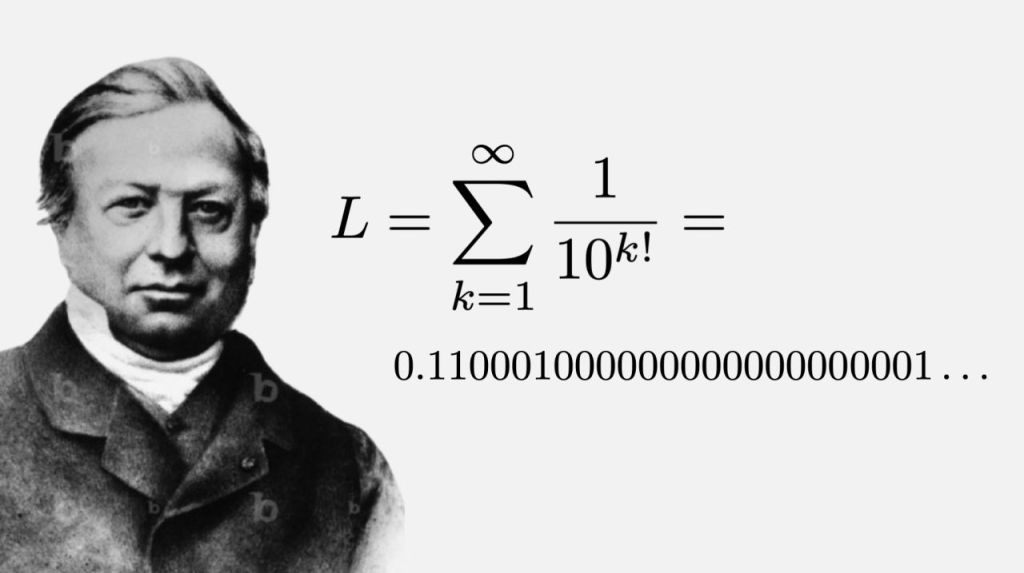


![\mathbb{Z}[x]](https://s0.wp.com/latex.php?latex=%5Cmathbb%7BZ%7D%5Bx%5D&bg=ffffff&fg=444444&s=0&c=20201002)


 belonging to
  or a more general topological vector space and its “dual” or “conjugate” function, defined on the dual space of linear forms. From a more practical perspective, it can be understood as an alternative way of encoding the information contained in a function. In that sense, it is very similar to other transforms like the Fourier series/transform and the Laplace transform. The Fourier series, for instance, encodes the information about the given (periodic) function in the form of a sequence of “amplitudes” corresponding to the different “modes”. The Fourier transform furnishes a similar integral representation for non-periodic functions, where this time different “modes” or “frequencies” form a continuum. Both the series and the transform provide a spectral representation of the function.
 is twice differentiable and
  for all
  with
with  , exponential functions
  with
with  , the function
  , etc.
 is a strictly increasing (hence one-to-one) function. Such correspondence allows to identify
  . In other words,
  can be used as a new independent variable. At this point, one might be tempted to use the function
  , where
  ) as an alternative representation of
  that has the following pleasant additional property: if the procedure is applied twice we recover the original function,
  . The transformation
  is what is called involutive (an involution).
 axis starting from
  . Assuming that
  , there will be a first point of contact with the graph of
  – axis; more precisely, if our line has equation
  , we define
  . The knowledge of the function
  at
at  and
and  are represented.
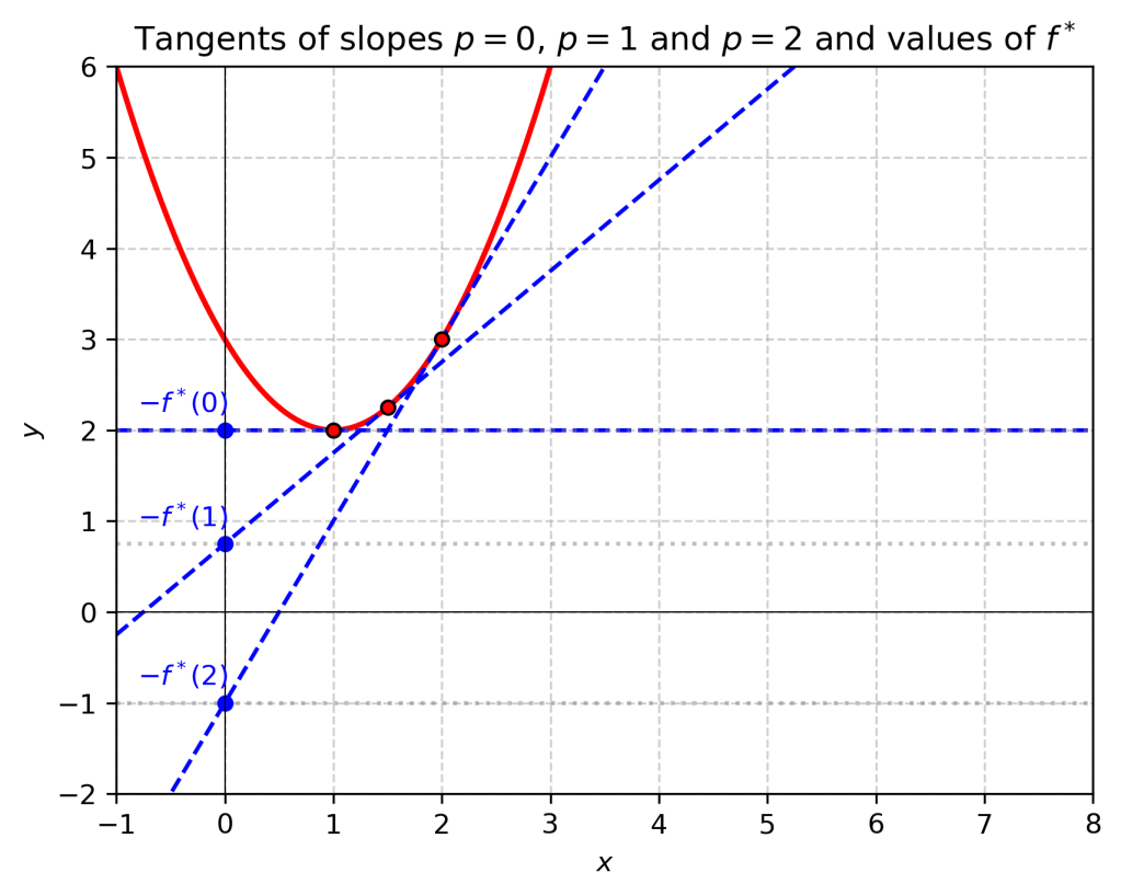
 in the equation
 . Its
. Its  . Finally,
 .
. .
.
 . The formula above reveals that
  , (i.e. the transformation is involutive), since
![\displaystyle{\frac{df^*(p)}{dp}=x(p)+p\frac{dx}{dp}-f'(x(p))\frac{dx}{dp}=x(p)+\frac{dx}{dp}\left[p-f'(x(p))\right]=x(p)}](https://s0.wp.com/latex.php?latex=%5Cdisplaystyle%7B%5Cfrac%7Bdf%5E%2A%28p%29%7D%7Bdp%7D%3Dx%28p%29%2Bp%5Cfrac%7Bdx%7D%7Bdp%7D-f%27%28x%28p%29%29%5Cfrac%7Bdx%7D%7Bdp%7D%3Dx%28p%29%2B%5Cfrac%7Bdx%7D%7Bdp%7D%5Cleft%5Bp-f%27%28x%28p%29%29%5Cright%5D%3Dx%28p%29%7D&bg=ffffff&fg=444444&s=0&c=20201002)
 . This point is a global maximum. Thus,
 .
.
 . Equality takes place when
  ,
,  . More generally, if
  with
with  for
for  , then
  , where
  . If
. If  , then
  , etc.
 in the range of
  , however, is not completely satisfactory for non-convex functions, as it loses information about the original function. However, for a convex function defined on
  ,
,  , a fact known as the Fenchel-Moreau theorem, [3]. Namely,
 ,
, , an extra technical condition is needed on
  to hold, namely lower semicontinuity, which is equivalent to the closedness of its epigraph. It is easy to see that this is a necessary condition for
  , then clearly
  , with
  . If
. If  when
when  and
and  when
when  , with
  and
and  , then
 ![p\in [a_1,a_2]](https://s0.wp.com/latex.php?latex=p%5Cin+%5Ba_1%2Ca_2%5D&bg=ffffff&fg=444444&s=0&c=20201002) , where it is linear and ranges from
, where it is linear and ranges from  to
to  . In general, to each “corner” of a polygonal graph there corresponds a segment on the graph of
  is straightforward. Under the smoothness and strict convexity assumption
 ,
,  is one-to-one. If
  via the standard Euclidean structure, we define the Legendre transform by
 ,
, denotes the inner product. Much like in the one-dimensional case, the previous definition is equivalent to
  .
. ,
,![f^*:\mathbb{R}^n\to (-\infty,+\infty]](https://s0.wp.com/latex.php?latex=f%5E%2A%3A%5Cmathbb%7BR%7D%5En%5Cto+%28-%5Cinfty%2C%2B%5Cinfty%5D&bg=ffffff&fg=444444&s=0&c=20201002) . The Fenchel-Moreau theorem holds without modifications under the extra assumption of lower semicontinuity of
. The Fenchel-Moreau theorem holds without modifications under the extra assumption of lower semicontinuity of  is a function of two variables, one can consider its transform with respect to the first variable,
 .
. , the supremum is achieved at the (unique)
  defined by
  .
. and their “conjugates” or “dual” on the cotangent bundle
  . Namely, the transform connects functions of
  with functions of
  , where
  and
and  .
. is Clairaut’s equation
 .
. as solutions. The envelope of the family is a singular solution satisfying
  . But these are precisely the relations defining the Legendre transform of
  on its configuration space (a differentiable, Riemannian manifold) completely describes the system. The actual path
  joining two states
  and
and  is an extremal of the action functional,
![S[q]=\displaystyle{\int\limits_{t_1}^{t_2}} L(q,\dot{q},t)\,dt](https://s0.wp.com/latex.php?latex=S%5Bq%5D%3D%5Cdisplaystyle%7B%5Cint%5Climits_%7Bt_1%7D%5E%7Bt_2%7D%7D++L%28q%2C%5Cdot%7Bq%7D%2Ct%29%5C%2Cdt&bg=ffffff&fg=444444&s=0&c=20201002)
 .
.  ,
,
 ,
, is the generalized momentum, an element of the cotangent fiber at
  . Since

 satisfy the first order Hamiltonian system:
 is called the phase space, and the Hamiltonian function equips it with a remarkable symplectic structure. The Hamiltonian flow (if
  does not depend on time) is a one-parameter subgroup of the group of symplectomorphisms of the phase space. A straightforward consequence is Liouville’s Theorem on the preservation of the phase volume (a cornerstone of Statistical Mechanics) . The Lagrangian approach has, however, certain advantages including: a) it is easier to deal with constraints, even non-holonomic via Lagrange multipliers; b) it is easier to track conserved quantities via Noether’s theorem, c) non-conservative forces can be incorporated, etc.
 is usually a positive definite quadratic function (the kinetic energy of the system) hence convex. The transform of a quadratic form is especially simple: it is just another quadratic form of the conjugate variable. For instance, the Lagrangian of a simple mass-spring system, assuming that the spring is linear and

 (internal energy) such that, for any thermodynamical system undergoing an infinitesimal change of state,
 ,
, represent the heat (thermal energy) added to the system,
  is the work of the surroundings on the system and the last sum above accounts for the energy added to the system by means of particle exchange. Here,
  is the amount of particles of the
  -th type added to the system, and
  the corresponding chemical potential. The relevant fact here is that
  is an actual differential, whereas the rest of the terms are just differential forms in the configuration space of the system. The term
  involving intensive (
 ) and conjugate extensive variables
  . Thus, for example, in the case of a gas expanding/compressing against the environment, the work done on the gas is
  , where
  is the infinitesimal change of volume and
  is the external pressure. Moreover, according to the second principle, for reversible processes the form
  , namely there is a function of state called entropy
  such that

 is the pressure of the gas in equilibrium with its surroundings.
  at pressure
  .
. we have
  ,
,  .
.  we have
 . Thus, the change of enthalpy determines if a given chemical reaction is exothermic or endothermic. Moreover,
  and
and  .
. ,
, ,
, as the pressure-volume work on the system under fixed temperature.
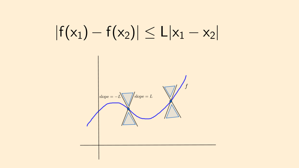

 is Lipschitz continuity of
  where
where  such that
 in
in ![\left\{\begin{array}{l}\displaystyle{ \frac{dx}{dt}=f(t,x)} ;\\[10pt] x(t_0)=x_0 \end{array}\right.\qquad\qquad\qquad \textrm{(IVP)}](https://s0.wp.com/latex.php?latex=%5Cleft%5C%7B%5Cbegin%7Barray%7D%7Bl%7D%5Cdisplaystyle%7B+%5Cfrac%7Bdx%7D%7Bdt%7D%3Df%28t%2Cx%29%7D+%3B%5C%5C%5B10pt%5D+x%28t_0%29%3Dx_0+%5Cend%7Barray%7D%5Cright.%5Cqquad%5Cqquad%5Cqquad+%5Ctextrm%7B%28IVP%29%7D&bg=ffffff&fg=444444&s=0&c=20201002)
 coincide in their intersection. We assume that our solutions are classical,
  , continuously differentiable. Such solutions exist when extra conditions on
  and
and  . We will also assume that
  for every
  and, therefore, one solution of the above IVP is
  . The general case reduces to this one, as we explain later.
 with
with  for some
  can never be zero at
  . We will assume
  , as the case
  can be handled in a similar way. Backwards uniqueness also follows easily from the forward result.
  to zero,
  ,
,  , while
  for
for  . By the Lipschitz condition,

 . Integrating this inequality over
 ![[t,t_1]](https://s0.wp.com/latex.php?latex=%5Bt%2Ct_1%5D&bg=ffffff&fg=444444&s=0&c=20201002) ,
,
 , contradicting the assumption
  as
as  . The Lipschitz condition prevents
  for some
  for some
  for all
  in its domain, thus preventing
 of the IVP
![\left\{\begin{array}{l}\displaystyle{ \frac{dy}{dt}=Ly} ;\\[10pt] y(t_1)=x_1 \end{array}\right.](https://s0.wp.com/latex.php?latex=%5Cleft%5C%7B%5Cbegin%7Barray%7D%7Bl%7D%5Cdisplaystyle%7B+%5Cfrac%7Bdy%7D%7Bdt%7D%3DLy%7D+%3B%5C%5C%5B10pt%5D+y%28t_1%29%3Dx_1+%5Cend%7Barray%7D%5Cright.&bg=ffffff&fg=444444&s=0&c=20201002)
 to the left of
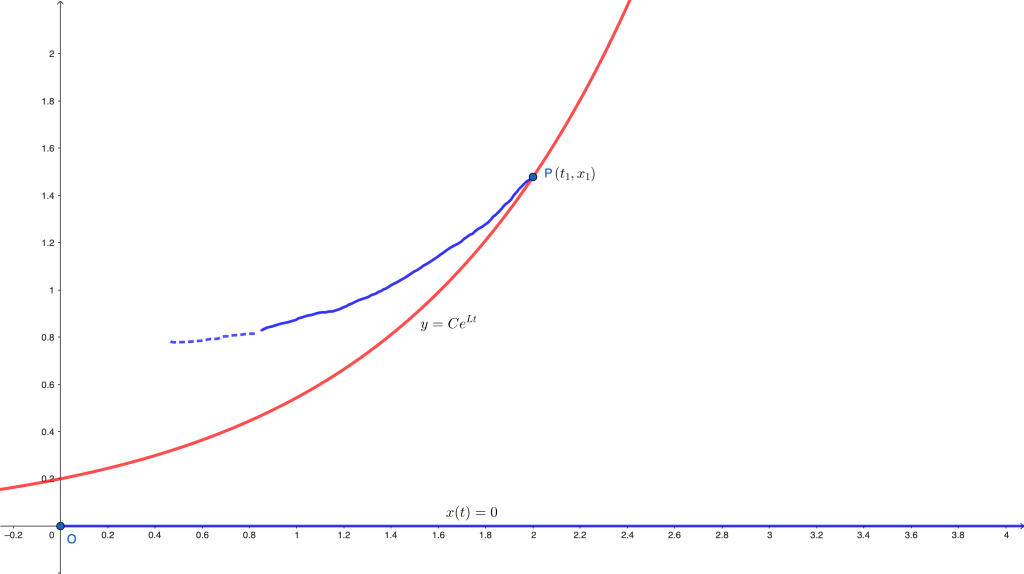
 from reaching the
  )
) 
 to conclude that
  with
with  is a barrier from above for our solution, preventing it from reaching the
  suggests a very natural generalization. Indeed, all we need is a diverging (at zero) improper integral on the right-hand side. We can replace the Lipschitz condition by the existence of a modulus of continuity, that is a continuous function
  with
with  ,
,  for
for  satisfying
 .
. . The proof is identical to the one above, given that the only property we need is the divergence of the improper integral of
  at
at  .
. that leads to a convergent improper integral. This condition is satisfied, for instance, in the autonomous problem
![\left\{\begin{array}{l}\displaystyle{ \frac{dx}{dt}=x^{2/3}} ;\\[10pt] x(0)=0 \end{array}\right.](https://s0.wp.com/latex.php?latex=%5Cleft%5C%7B%5Cbegin%7Barray%7D%7Bl%7D%5Cdisplaystyle%7B+%5Cfrac%7Bdx%7D%7Bdt%7D%3Dx%5E%7B2%2F3%7D%7D+%3B%5C%5C%5B10pt%5D+x%280%29%3D0+%5Cend%7Barray%7D%5Cright.&bg=ffffff&fg=444444&s=0&c=20201002)
 on
on  and
and  for
for  for any
  .
. in this example. Any power
  would do. These examples of non-uniqueness are usually attributed to G. Peano.
 and
and  are local solutions of
  ), then
  is a local solution of
![\left\{\begin{array}{l}\displaystyle{ \frac{d\bar x}{ds}=g(s,\bar x):=f(s+t_0, \bar x+x_1(s+t_0))-f(s+t_0, x_1(s+t_0))} ;\\[10pt] \bar x(0)=0 \end{array}\right.](https://s0.wp.com/latex.php?latex=%5Cleft%5C%7B%5Cbegin%7Barray%7D%7Bl%7D%5Cdisplaystyle%7B+%5Cfrac%7Bd%5Cbar+x%7D%7Bds%7D%3Dg%28s%2C%5Cbar+x%29%3A%3Df%28s%2Bt_0%2C+%5Cbar+x%2Bx_1%28s%2Bt_0%29%29-f%28s%2Bt_0%2C++x_1%28s%2Bt_0%29%29%7D+%3B%5C%5C%5B10pt%5D+%5Cbar+x%280%29%3D0+%5Cend%7Barray%7D%5Cright.&bg=ffffff&fg=444444&s=0&c=20201002)
 with
with  . Moreover,
  satisfies a Lipschitz condition near
  if
if  and hence
  on the corresponding intervals.
 A simple and widely used sufficient condition for
  in an
in an 
 with
with  with
with ![\alpha\in (0,2]](https://s0.wp.com/latex.php?latex=%5Calpha%5Cin+%280%2C2%5D&bg=ffffff&fg=444444&s=0&c=20201002) shows;
shows;  The Lipschitz condition is relevant in other areas of Analysis. For instance, it guarantees the uniform convergence of Fourier series.
 as
as  , assuming that the domain of definition of
 ![\left\{\begin{array}{l}\displaystyle{ \frac{dx}{dt}=x^2} ;\\[10pt] x(t_0)=x_0>0 \end{array}\right.](https://s0.wp.com/latex.php?latex=%5Cleft%5C%7B%5Cbegin%7Barray%7D%7Bl%7D%5Cdisplaystyle%7B+%5Cfrac%7Bdx%7D%7Bdt%7D%3Dx%5E2%7D+%3B%5C%5C%5B10pt%5D+x%28t_0%29%3Dx_0%3E0+%5Cend%7Barray%7D%5Cright.&bg=ffffff&fg=444444&s=0&c=20201002) ,
, “blows up” as
  , despite the fact that
  is smooth on the whole plane. The role of the superlinear growth at infinity is similar to the role of Lipschitz (or Osgood) condition in bounded regions for uniqueness. The above problem is equivalent to
 prevents
  , we have
  . This phenomenon is called finite time blow-up and is exhibited by ODEs with superlinear right-hand-sides, by some evolution PDEs with superlinear sources, etc.
 such that
  as
as  (resp.
  as
as  ) if only
 .
. stays to the left of the solution of
![\left\{\begin{array}{l}\displaystyle{ \frac{dx}{dt}=\Psi(x)} \\[10pt] x(t_0)=x_0 \end{array}\right.](https://s0.wp.com/latex.php?latex=%5Cleft%5C%7B%5Cbegin%7Barray%7D%7Bl%7D%5Cdisplaystyle%7B+%5Cfrac%7Bdx%7D%7Bdt%7D%3D%5CPsi%28x%29%7D+%5C%5C%5B10pt%5D+x%28t_0%29%3Dx_0+%5Cend%7Barray%7D%5Cright.&bg=ffffff&fg=444444&s=0&c=20201002)
 . The latter blows up in finite time, namely at time
  , forcing the solution to our IVP to blow up at some
  .
.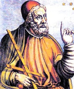
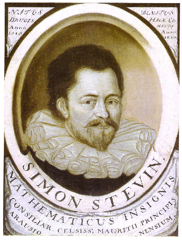

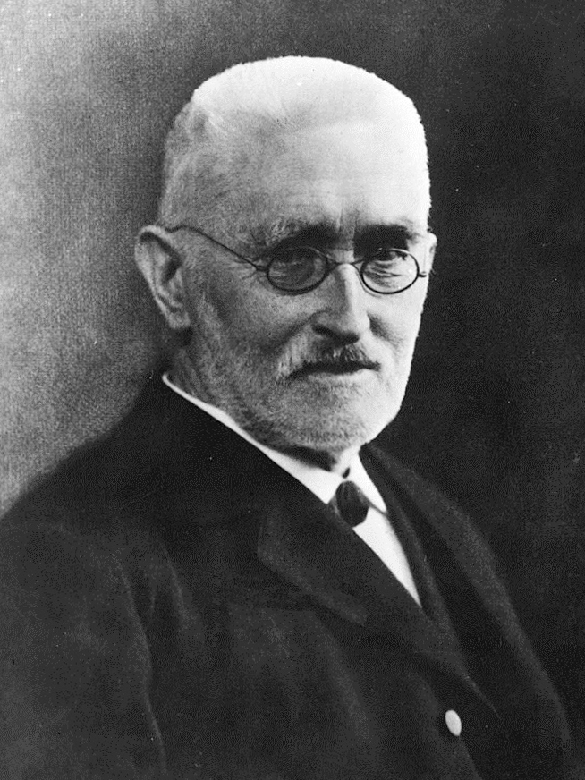
 ) are built.
  , makes correspond, if
  , a multiple of
  we say that the first is to the second as the third is to the fourth,
  if, for any integers
  the following equivalencies hold
 ,
, and
and  are commensurable, there exist integers
  and
and  . But again, neither those rational approximations or the final ratio were “numbers”.
 ,
,  etc. Bombelli is also responsible for an early use of “imaginary” numbers for the solution of cubic equations.
 with the property
 ,
, as
as  , the other case being completely analogous. When
  we say that the asymptote is horizontal. A simple way to detect if a given function has a slant asymptote is by checking linearity at infinity,
  if the limit
 ,
,
 are polynomials, the situation is much simpler. In order for
  and, if that is the case, we perform long division which leads to
 and, therefore, the asymptote is just the quotient
 , the fraction is superlinear at infinity.
  does not require derivatives at all. In order to understand this, we notice that
  is a tangent to
  at
at 
 as
as  . The last relation is very similar to
  ,
, 
 ,
,  with first partial remainder
  . In the next step, we add
  to the quotient, with a partial remainder
  . Since we are interested in the tangent line and
  is an infinitesimal of degree higher than one at zero, the division stops here and the equation of the tangent is
  . If we keep dividing, we get the Taylor polynomials of higher degree. For instance, the osculating parabola at
  and so on.
  in the decimal representation of numbers by
  at
at  , all we need to do is set
  and express
  and then finding the tangent at
  as before. Finally, we have to replace
  in the found equation of the tangent.
 by
by  is performed in order to get the power series expansion.
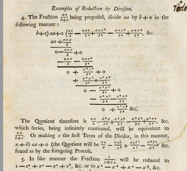


 ,
,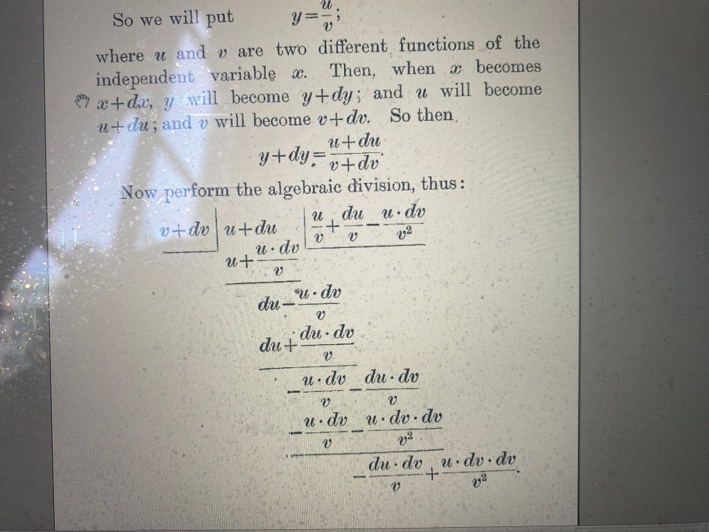

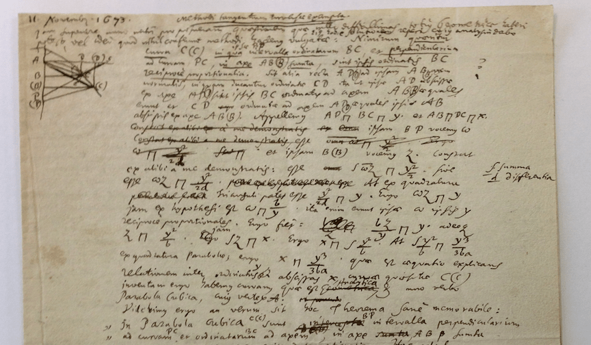
 for sums. He uses the sign
  for adequalities). In the hands of the Bernoullis, Huygens, Euler, Lagrange, Legendre and many others, Infinitesimal Calculus, including the theory of differential equations as well as numerous applications to Mechanics, Optics, etc. developed for over 150 years under that conceptual framework. The situation changed during the second half of the XIX century, when set theory and a rigorous construction of the continuum was put forward by Cantor and Dedekind. Supposedly, they provided a final answer to the nature of the continuum that has been prevalent for over 150 years by now. Such a sparse ontology did not convince everyone, and there have been numerous alternative models of the continuum developed over time, aimed at restoring the language of infinitesimals, see [1]. As for the concepts of derivative and integral, infinitesimal interpretations were replaced by epsilons and deltas at the hands of Bolzano, Cauchy and, notably, Weierstrass.
 , if
, if  , we say that
  if for any
  there exists some
  such that

![[a,b]](https://s0.wp.com/latex.php?latex=%5Ba%2Cb%5D&bg=ffffff&fg=444444&s=0&c=20201002) , we consider partitions
, we consider partitions  , where
  with tags
 ![\xi_i\in [x_{i-1},x_i]](https://s0.wp.com/latex.php?latex=%5Cxi_i%5Cin+%5Bx_%7Bi-1%7D%2Cx_i%5D&bg=ffffff&fg=444444&s=0&c=20201002) and form the Riemann sums
and form the Riemann sums .
. as
as  (uniformly w.r.t. the partitions and the tags), we say that
  there exists
  such that
 , one has to travel half of the distance, then a fourth of the distance, then an eight of it, etc. Zeno rejected the possibility of such process made of infinitely many steps since, in his opinion, it could never be completed. Thus for Zeno and the followers of Parmenides, motion did not exist. Greek mathematics rejected completed infinite processes in general (see [2]) and therefore could not attach a numerical value to the “infinite sum”

 , and then noticing that
  “stabilizes towards
  “, and thus has the real number
  in this example, the sum happens to be a rational number, but the concept of real number allows to attach a sum to series like
 .
.  to have a finite sum in the above sense is that the general term of the sequence converge to zero,
  . Indeed, if
  has to vanish asymptotically. The elementary theory of numerical series shows that this condition is not sufficient and that there are two main mechanisms of convergence:
  .
.  , thus balancing the number of addends
  the terms become arbitrarily small simultaneously, allowing for a “larger” number of addends, namely the continuous sum
![I=[a,b]](https://s0.wp.com/latex.php?latex=I%3D%5Ba%2Cb%5D&bg=ffffff&fg=444444&s=0&c=20201002) . We can think of
. We can think of  as the infinitesimal addends making up the sum. The situation here is more delicate, since all the terms making up the Riemann sums change every time and the values of the sums may not stabilize if the function is too discontinuous. Everything works nicely for continuous functions though.
 , he/she reasons as follows: choose an infinitesimal portion of the bar of length
  between two infinitesimally close points
  . Being infinitesimal, the density is constant and equal to
  . The total mass is thus the sum of the infinitesimal masses
 .
.

 as
as  .
.![I=[a,b]\times[c,d]](https://s0.wp.com/latex.php?latex=I%3D%5Ba%2Cb%5D%5Ctimes%5Bc%2Cd%5D&bg=ffffff&fg=444444&s=0&c=20201002) . Those are double integrals
. Those are double integrals![\displaystyle{\iint\limits_{[a,b]\times[c,d]} f(x,y)\, dxdy}](https://s0.wp.com/latex.php?latex=%5Cdisplaystyle%7B%5Ciint%5Climits_%7B%5Ba%2Cb%5D%5Ctimes%5Bc%2Cd%5D%7D+f%28x%2Cy%29%5C%2C+dxdy%7D&bg=ffffff&fg=444444&s=0&c=20201002) ,
, with respect to
  . The same applies to general multiple integrals. Unbalanced Riemann sums give rise to trivial objects like
![\displaystyle{\iint\limits_{[a,b]\times[c,d]}f(x,y)\,dx^2dy=0};\qquad\displaystyle{\iiint\limits_{[a,b]\times [c,d]\times [e,f]}f(x,y,z)\,dxdz=\infty}](https://s0.wp.com/latex.php?latex=%5Cdisplaystyle%7B%5Ciint%5Climits_%7B%5Ba%2Cb%5D%5Ctimes%5Bc%2Cd%5D%7Df%28x%2Cy%29%5C%2Cdx%5E2dy%3D0%7D%3B%5Cqquad%5Cdisplaystyle%7B%5Ciiint%5Climits_%7B%5Ba%2Cb%5D%5Ctimes+%5Bc%2Cd%5D%5Ctimes+%5Be%2Cf%5D%7Df%28x%2Cy%2Cz%29%5C%2Cdxdz%3D%5Cinfty%7D&bg=ffffff&fg=444444&s=0&c=20201002) ,
, definition of the definite integral. They help understand why the concept of definite integral is relevant as it strikes the sweet spot where the “number of addends” (i.e. the cardinality of the set of indices) and their size balance each other, resulting in convergence to a finite, nontrivial sum.
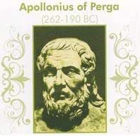
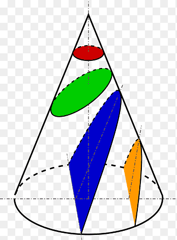
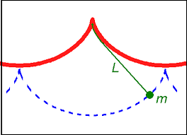
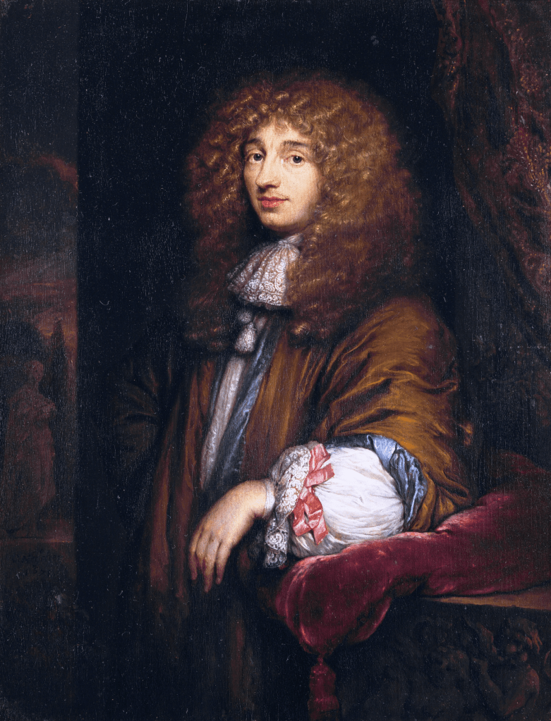
 . In other words, it is the locus of points equidistant from the focus and the directrix. A two line computation gives the equation
 and directrix
  . In a similar fashion the equations for the other conics can be obtained and used to derive further properties. Conic sections correspond to quadratic equations in two variables, a fact first established by Wallis in 1655.
 etc. which can be integrated in quadratures in some cases.
  at a generic point of the sought after curve was (and still is) a valuable tool in the derivation of the differential relations. Let’s look into some examples.
 – plane satisfying the following property: the area of the triangle defined by the tangent, the ordinate and the subtangent is a positive constant
  , its ordinate by
  and the subtangent be
  (figure below).
 is tangent to the curve, the triangle
  is similar to the differential triangle at


 ,
, . As we move along one of these hyperbolas, the distance to the
  -axis is inversely proportional to the size of the subtangent.
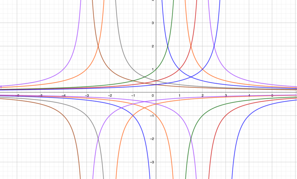
 -axis containing the point where the object is initially located. Let
  . We look at this problem from a strictly geometric point of view, assuming that the object is a mass point that reacts instantly to the pulling force, aligning its motion with the force at all times. In other words, the goal is to find a curve whose segment of tangent between the point of tangency and the
  is the foot of the perpendicular from
  is the abscissa). Here,
  .
.
 .
. 
 .
. then reads
 ,
, ) adding the condition
  gives
gives
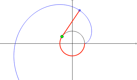
 ,
, (if we think of the parameter
  the coordinates of the point of the involute on the tangent to
  and let
  the length of the detached portion of the string (that is, the arc length measured from the point of detachment, also called natural parameter in Differential Geometry). In the figure below, we assume that the base curve is positively oriented, so the increase of the parameter
  . The string is also being unwrapped counterclockwise.
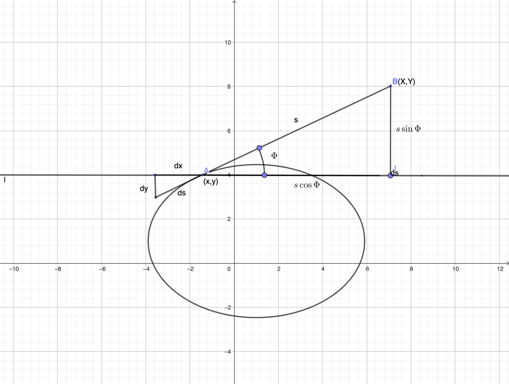
 ,
, is the angle formed by the tangent at
  .
.  .
.  .
. , clearly
  if we choose the point
  as the starting point. An appplication of the general formula gives
 and
and  . It is representative of the Leibnizian calculus of infinitesimals. Remarkably, the result involves second differentials.
 be a portion of a regular curve, with
  and
and  being infinitesimally close points on it. Let the normals to the curve at
  and pick the
  and
and  at points
  . We draw a vertical auxiliary line
  and a horizontal line through
  , and yet another vertical through
  at
at  . Finally, we draw
  , perpendicular to
  (resp.
  ). Our goal is to compute the radius of curvature
  , in terms of
  ,
,  and their differentials
  and
and  . Due to the local nature of
  directly.
 ,
,  ,
,  are all similar (strictly or up to negligible infinitesimals) to the differential triangle
  . From the similarity of
  and
and  we get
 and solving for
  .
. ;
; ;
; .
. .
. (otherwise the point
  we obtain the familiar formula
 .
. , the osculating circle degenerates into a line and
  .
. above. Since
  one has
 ,
, ,
, on the evolute by shifting the point
  by the amount
  .That is,
  .
. , multipliées chacune par un coefficient indéterminé qu’ensuite on égale à zéro la somme de tous les terms qui se trouvent multipliés par une même différentielle… – J. L. Lagrange, “Méchanique Analytique”.
 and therefore their gradients have to be collinear. Despite how appealing this interpretation might be, it does not correspond to the historical development of the method. It is rather an afterthought. A similar example would be motivating Pythagorean theorem using vectors and the inner product in
  . I believe that re-interpreting mathematical facts from a higher perspective is very useful but using those re-interpretations as motivation is misleading.
 ,
,  . Let the total force acting on the
  . If there are no constraints on the particles, all possible displacements
  are admissible and, according to the principle of virtual displacements, the system is in equilibrium if and only if
 . By freezing all of the
  ‘s but one, we see that each of the addends in the above sum has to vanish, that is
 .
.  are arbitrary, this in turn implies
 ,
, ,
, – dimensional space and therefore to their (generically)
  – dimensional intersection, a manifold in
  . To calculate those virtual displacements, we differentiate each one of the above equations, yielding
![\left\{\begin{array}{l}\displaystyle{\frac{\partial g_1}{\partial \mathbf{r}_1}\cdot d\mathbf{r}_1+\frac{\partial g_1}{\partial \mathbf{r}_2}\cdot d\mathbf{r}_2+\dots \frac{\partial g_1}{\partial \mathbf{r}_N}\cdot d\mathbf{r}_N=0}\\ [15pt]\displaystyle{\frac{\partial g_2}{\partial \mathbf{r}_1}\cdot d\mathbf{r}_1+\frac{\partial g_2}{\partial \mathbf{r}_2}\cdot d\mathbf{r}_2+\dots \frac{\partial g_2}{\partial \mathbf{r}_N}\cdot d\mathbf{r}_N=0}\\[15pt]\cdots\cdots\cdots\cdots\end{array}\qquad\qquad\qquad\quad (2)\right.](https://s0.wp.com/latex.php?latex=%5Cleft%5C%7B%5Cbegin%7Barray%7D%7Bl%7D%5Cdisplaystyle%7B%5Cfrac%7B%5Cpartial+g_1%7D%7B%5Cpartial+%5Cmathbf%7Br%7D_1%7D%5Ccdot+d%5Cmathbf%7Br%7D_1%2B%5Cfrac%7B%5Cpartial+g_1%7D%7B%5Cpartial+%5Cmathbf%7Br%7D_2%7D%5Ccdot+d%5Cmathbf%7Br%7D_2%2B%5Cdots+%5Cfrac%7B%5Cpartial+g_1%7D%7B%5Cpartial+%5Cmathbf%7Br%7D_N%7D%5Ccdot+d%5Cmathbf%7Br%7D_N%3D0%7D%5C%5C+%5B15pt%5D%5Cdisplaystyle%7B%5Cfrac%7B%5Cpartial+g_2%7D%7B%5Cpartial+%5Cmathbf%7Br%7D_1%7D%5Ccdot+d%5Cmathbf%7Br%7D_1%2B%5Cfrac%7B%5Cpartial+g_2%7D%7B%5Cpartial+%5Cmathbf%7Br%7D_2%7D%5Ccdot+d%5Cmathbf%7Br%7D_2%2B%5Cdots+%5Cfrac%7B%5Cpartial+g_2%7D%7B%5Cpartial+%5Cmathbf%7Br%7D_N%7D%5Ccdot+d%5Cmathbf%7Br%7D_N%3D0%7D%5C%5C%5B15pt%5D%5Ccdots%5Ccdots%5Ccdots%5Ccdots%5Cend%7Barray%7D%5Cqquad%5Cqquad%5Cqquad%5Cquad+%282%29%5Cright.&bg=ffffff&fg=444444&s=0&c=20201002)

 for all
  independent ones and substitute into
  . Then
  ,
, , etc. are the partial derivatives of some function
  has to be non-zero if
  and add it to the first. Thus at any given point we can choose

 , we get the equilibria.
 and add their sum to
  . We choose the multipliers in order to remove
  , otherwise no freedom is left for the system. For example, one particle in space can be subject to lie on a surface or on a line (the intersection of two surfaces). Adding one more constraint would completely fix its position.
  . When the work of a force can be put in the form
  ,
,
 stands for the mass of the
  for its acceleration.
![\left\{\begin{array}{l}-mx''+F_x+\lambda\frac{\partial g}{\partial x}=0\\[15pt]-my''+F_y+\lambda\frac{\partial g}{\partial y}=0\\[15pt]-mz''+F_z+\lambda\frac{\partial g}{\partial z}=0\end{array}\right.](https://s0.wp.com/latex.php?latex=%5Cleft%5C%7B%5Cbegin%7Barray%7D%7Bl%7D-mx%27%27%2BF_x%2B%5Clambda%5Cfrac%7B%5Cpartial+g%7D%7B%5Cpartial+x%7D%3D0%5C%5C%5B15pt%5D-my%27%27%2BF_y%2B%5Clambda%5Cfrac%7B%5Cpartial+g%7D%7B%5Cpartial+y%7D%3D0%5C%5C%5B15pt%5D-mz%27%27%2BF_z%2B%5Clambda%5Cfrac%7B%5Cpartial+g%7D%7B%5Cpartial+z%7D%3D0%5Cend%7Barray%7D%5Cright.&bg=ffffff&fg=444444&s=0&c=20201002)

 The above method can be applied if the constraints are time-dependent (rheonomic). Precisely, if we have just one particle and a constraint of the form
 , virtual displacements
  satisfy the same equation as before (second equation in
  linear in the velocities). See [3].
 Holonomic constraints can be completely eliminated by introducing independent generalized coordinates which implicitly account for them. Thus if
  ,
,  are generalized coordinates of the system and its kinetic energy is
  , we can write the equations of motion in the (Lagrangian) form
 ,
, are generalized forces, [3]. By solving this second order system of equations we find the dynamics
  . But in some cases we are interested in the forces of constraint. One way to find them would be to substitute into Newton’s second law and solving for the unaccounted forces. However, it is generally more convenient to use dependent generalized coordinates in combination with the method of multipliers to deal with constraints and find the forces of constraint as above.
  If all the constraints are holonomic and forces are conservative with potential energy
![\displaystyle{S[\mathbf{q}]=\int\limits_{t_1}^{t_2}L(\mathbf{q}',\mathbf{q},t)\,dt}](https://s0.wp.com/latex.php?latex=%5Cdisplaystyle%7BS%5B%5Cmathbf%7Bq%7D%5D%3D%5Cint%5Climits_%7Bt_1%7D%5E%7Bt_2%7DL%28%5Cmathbf%7Bq%7D%27%2C%5Cmathbf%7Bq%7D%2Ct%29%5C%2Cdt%7D&bg=ffffff&fg=444444&s=0&c=20201002) ,
, are, as before, generalized coordinates on the
  – dimensional manifold
  defined by the constraints,
  is the kinetic energy and
  is the Lagrangian of the system. The true motion
  .
. particles is straightforward.
 by their perturbed values
  and disregard infinitesimals which are of order higher than one with respect to
  in the resulting expression.
  for some constants
  , we have
 ,
, . In this case, the expression is linear in
  and
and  and, therefore
 .
. , we notice that
 , we get
  .
.

 ,
,
 ,
, . Finally, since
  we get
 .
.
 . For negative integer powers the same rule applies, as follows from the quotient and power rules. Combining the previous, we can differentiate any equation involving polynomial or rational functions.
 . In modern textbooks, they focus on the derivative
  . The computation goes more or less like this.
 ,
, as
as  . All this is nice and clean but does not provide compelling intuition. Next, we provide a proof based on infinitesimals. No computation needed. It is essentially a picture-based proof.
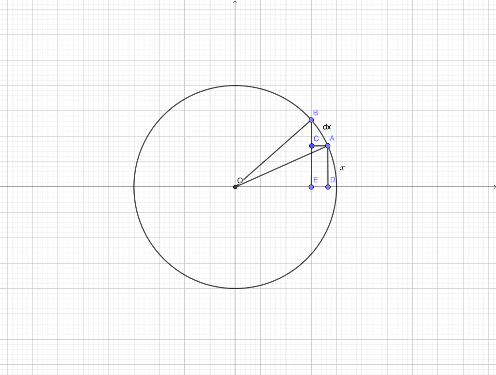
 is
is  . The triangles
  and
and  are similar since they are right and
  . Therefore,
 .
. is actually
  , etc. BUT it provides a visual, compelling reason as to why
  and the conclusion is absolutely correct. It is correct because we know that the vanishing circular arc
  is indistinguishable from its tangent, while
  .
.  . In the figure below,
  and
and  is right. Then
  . We increase the angle
  by an infinitesimal amount
  . The tangent is then increased by
  . Let
. Let  be the arc of a circle centered at
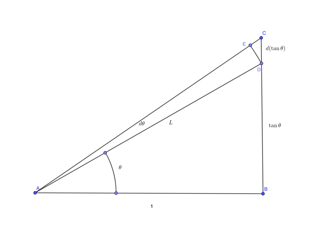
 are similar and thus

 differs from
  .
. and
and  be the lengths of the legs of the triangle. Then,

 . Thus we get a system of equations
 are allowed) we need zero determinant,
  which in our case implies
  and then, from our second finite relation we get
  .
. and substitute, leading to the problem of minimizing a function of
 and set it equal to zero. In this simple example there is no big difference, but notice that with our approach: a) no “independent variable” is singled out; b) we avoid the annoyance of taking the derivative of a square root; c)
 ,
,  . This problem involves more parameters and, no matter what quantity you choose as independent, the solution using derivatives is a bit messy. Using differentials, it reduces to a compatibility condition for a homogeneous linear system as above. Namely, we have
 .
.
 . Replacing
  and
and  in terms of
  and
and  we end up with a
  system for
  :
:
 . This in turn implies
 . Finally,
 .
. so the path should “reflect” on the line.
 .
. ,
, . During the XVII and XVIII centuries, mathematicians thought of
  , which plays a central role, and both
  , linear in its second argument.
  is true by definition. This point of view stresses the notion of derivative, rendering differentials as superfluous, some sort of annoyance of the past, used only in the context of linear approximation, see [1].
 (respectively
  ) in a way consistent with the above relation,
 ,
, .
.
 is dropped. This is a general principle in Differential Calculus: in any computation involving infinitesimals, one should keep the leading ones (i.e. the ones of lowest order), dropping the higher order ones. This principle is followed by physicists, engineers and other users of differential calculus, and deemed as intuitively clear. It can be ultimately justified using the language of limits.
 in
in  ,
, . This approach carries some unpleasant consequences. For example, in modern notation
 on some interval. Thus, the function
  on the interval
  is a solution of (3). The function
  on the same interval is also a solution. But it would definitely be much nicer to be able to say that the full circle
  we started with is a solution to the symmetric differential equation
 . Then, the full set of solutions (to be precise, non-prolongable ones) is made of right, left, upper and lower half-circles. This is a consequence of insisting on functional relations and finite rates, where the variables play an asymmetric role. This was never an issue for Leibniz, Huygens, the Bernoullis, L’Hôpital or Euler. Much less for Newton, whose independent variable was always time, an extrinsic parameter. Equations in “differential form” like
  by
by  on the left hand side and impose
  up to infinitesimals of order higher than
  (quadratic, cubic, etc.) That leads to a differential relation
 (see below).
 respectively. For the sake of simplicity, assume there are two independent variables,
  and
and  . Then, if
  can be written in the form
 etc.) we say that
 and
and  are called partial derivatives of
 are compatible with
  to first order. Next, we present a nice geometric interpretation of the notion of compatibility.
 , contained in the domain of
 defines a hyperbola in the
  -plane, and the corresponding differential form is
  .
.  holds along
  to be perpendicular to the gradient vector
  which is in turn perpendicular to the level set
  .
.
 ……………………………………….
 ; it just needs to be tangent to the hyper-surface
  , we obtain a valid differential relation between the new variables by just considering