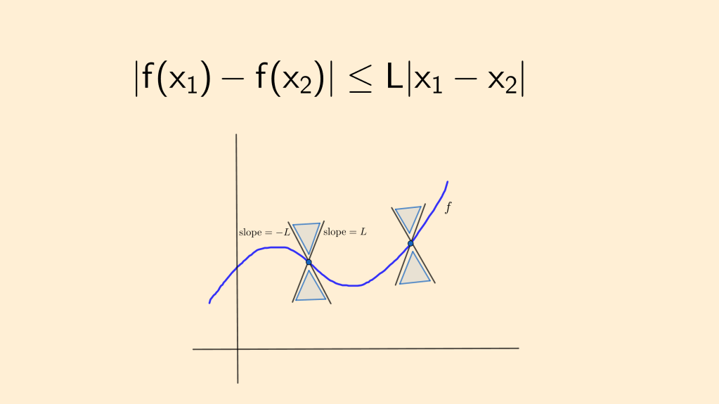
Fig.1. (L) The Lipschitz condition for a function . (R) Rudolph Lipschitz (1832 -1903)
A classic condition on the right hand side of a first order normal ODE
guaranteeing local uniqueness of solutions with given initial value is Lipschitz continuity of in the variable in some open, connected neighborhood of where is defined. That is, it is required that there exist some constant such that
for all in . Under the above condition there is a unique local solution of the initial value problem
where uniqueness means that two prospective solutions defined on open intervals containing coincide in their intersection. We assume that our solutions are classical, , continuously differentiable. Such solutions exist when extra conditions on are imposed. For instance, if is assumed continuous in , classical local solutions exist and can be extended up to the boundary of . But here our concern is uniqueness.
My goal here is to explain why such condition implies uniqueness in simple terms, how it can be generalized and the relation between uniqueness and another interesting phenomenon, namely finite-time blow-up of solutions.
To illustrate the idea, we will assume that and . We will also assume that for every and, therefore, one solution of the above IVP is . The general case reduces to this one, as we explain later.
We focus on forward uniqueness. Namely, we will prove that a solution with for some can never be zero at . We will assume , as the case can be handled in a similar way. Backwards uniqueness also follows easily from the forward result.
Uniqueness is violated if, as decreases from to zero, vanishes at some point , , while for . By the Lipschitz condition,
while . It then follows from the ODE that
along the solution for . Integrating this inequality over ,
This integral inequality is the crux of the argument. Just observe that, since the improper integral is divergent, approaching zero would require , contradicting the assumption as . The Lipschitz condition prevents from becoming zero over finite -intervals.
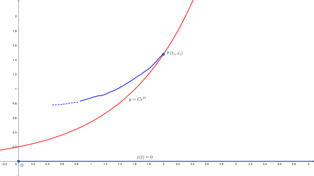
The argument above is equivalent to the following: for any solution with for some one can construct an exponential barrier from below of the form for some , that is, for all in its domain, thus preventing from becoming zero. Indeed, the inequality
implies that our solution is increasing at a slower pace than the solution of the IVP
which is nothing but for the appropriate . Therefore, to the left of . In other words, acts as a lower barrier for , as in the figure below.
Fig 2. The exponential barrier prevents the solution through from reaching the -axis.
If we assume that , we use the inequality (again a consequence of )
for to conclude that with is a barrier from above for our solution, preventing it from reaching the -axis.
The integral inequality suggests a very natural generalization. Indeed, all we need is a diverging (at zero) improper integral on the right-hand side. We can replace the Lipschitz condition by the existence of a modulus of continuity, that is a continuous function with , for satisfying
in , with the additional property
.
This more general statement is due to W. Osgood. The Lipschitz condition corresponds to the choice . The proof is identical to the one above, given that the only property we need is the divergence of the improper integral of at .
Thus, for an alternative solution to branch out from the trivial one, we require a non-Lipschitz right-hand side in that leads to a convergent improper integral. This condition is satisfied, for instance, in the autonomous problem
which, apart from the trivial solution, has solutions of the form on and for for any .
There is nothing special about the power in this example. Any power with would do. These examples of non-uniqueness are usually attributed to G. Peano.
Uniqueness for general solutions can be easily reduced to the special case above. Namely, if and are local solutions of (say on ), then is a local solution of
on with . Moreover, satisfies a Lipschitz condition near if does near , with the same constant . By the above particular result, and hence on the corresponding intervals.
Remarks: A simple and widely used sufficient condition for to hold is the continuity of the partial derivative in an -convex region (typically a rectangle). This follows from a straightforward application of Lagrange’s mean value theorem; is not necessary for uniqueness, as the example of with with shows; The Lipschitz condition is relevant in other areas of Analysis. For instance, it guarantees the uniform convergence of Fourier series.
A related phenomenon: blow up in finite time.
Local solutions issued from can be extended to the boundary of , but not necessarily in the -direction. The reason is a fast (superlinear) grow of as , assuming that the domain of definition of extends indefinitely in the -direction. A simple example is the problem
,
whose explicit solution “blows up” as , despite the fact that is smooth on the whole plane. The role of the superlinear growth at infinity is similar to the role of Lipschitz (or Osgood) condition in bounded regions for uniqueness. The above problem is equivalent to
Convergence of the improper integral prevents from attaining arbitrarily large values. Calling , we have . This phenomenon is called finite time blow-up and is exhibited by ODEs with superlinear right-hand-sides, by some evolution PDEs with superlinear sources, etc.
The same reasoning applies in the general case when there exists a continuous such that as (resp. as ) if only
.
This time, under assumptions guaranteeing existence and uniqueness of solutions and provided the first condition above holds, the (forward) solution to with stays to the left of the solution of
with . The latter blows up in finite time, namely at time , forcing the solution to our IVP to blow up at some .
Sets of points satisfying certain geometric condition are ubiquitous in Mathematics. The simplest examples are straight lines, circles and more general conics. Thus a straight line can be defined as the set of points equidistant from two given points, a circle as the set of points whose distance to a fixed point (center) is constant and a conic as the set of points such that the ratio of the distances to a given point (focus) and a given line (directrix) is constant. The type of conic depends on whether the ratio (called eccentricity) is less, equal or greater than one.
Straight lines and circles were intensively studied since antiquity. They were the favorite objects of Greek geometers, and their properties are thoroughly investigated in Euclid’s Elements. In his fundamental treatise “Conics”, Apollonius of Perga, known as the “Great Geometer”, went further, tackling a systematic study of conics, establishing their focal properties, as well as those of chords and tangents, “conjugate” diameters, asymptotes, etc. It is believed that he heavily drew from previous work by Euclid as well as from Menaechmus, who is generally considered the discoverer of conic sections.
Greeks did not stop there. For the purpose of solving construction problems not amenable to the straightedge and the compass, they introduced more sophisticated loci like conchoids and cissoids, and “kinematic” curves like the quadratrix or the Archimedean spiral.
When the method of coordinates was introduced by Fermat and Decartes in the XVII century, the sophisticated auxiliary constructions typical of synthetic geometry were replaced by more straightforward and systematic algebraic methods. The equations of the above mentioned curves were obtained right away by expressing their defining properties in the language of Algebra. For instance, a parabola is a conic with eccentricity . In other words, it is the locus of points equidistant from the focus and the directrix. A two line computation gives the equation
for a parabola with focus at and directrix . In a similar fashion the equations for the other conics can be obtained and used to derive further properties. Conic sections correspond to quadratic equations in two variables, a fact first established by Wallis in 1655.
Yet another locus, also considered by the Greeks, is that of points such that the ratio of their distances to two given points is constant. Using coordinates, one easily arrives at the equation of a circle (or a line if the ratio is equal to one). These are the so called Apollonian circles. They appear in applications, for instance as the zero-potential line for a system of two point charges in Electrostatics.
In the previous examples, the property defining the curve could be directly translated into a finite algebraic relation between the coordinates. With the birth of Calculus other classes of curves started to draw the attention of scholars, namely those whose defining property was more “local” in nature, in the sense that it involved the direction or some other feature of the curve at each point. In those cases, the defining property is not a finite, but rather a differential equation, relating etc. which can be integrated in quadratures in some cases.
The consideration of the “differential triangle” with sides at a generic point of the sought after curve was (and still is) a valuable tool in the derivation of the differential relations. Let’s look into some examples.
A family of equilateral hyperbolas
Consider the locus of points on the – plane satisfying the following property: the area of the triangle defined by the tangent, the ordinate and the subtangent is a positive constant .
Let the generic point be , its ordinate by and the subtangent be (figure below).
Since is tangent to the curve, the triangle is similar to the differential triangle at . Therefore,
and, consequently
The given condition then reads
or
The expression on the left is a total differential,
giving a general solution of the form
,
which is a family of equilateral hyperbolas with common asymptote . As we move along one of these hyperbolas, the distance to the -axis is inversely proportional to the size of the subtangent.
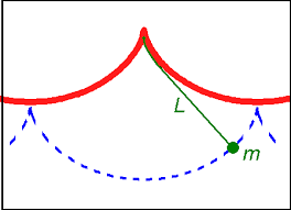
The tractrix
The following problem was proposed by Claude Perrault in1670, solved in 1692 by Huygens and subsequently solved by Leibniz, Johann Bernoulli and others.
“What is the path of an object dragged along a horizontal plane by a string of constant length when the end of the string not joined to the object moves along a straight line in the plane?”
Obviously, if the object is initially on the line of the force, the path is just a line. Assume it is not. For simplicity, choose the -axis in the direction of the force and the -axis containing the point where the object is initially located. Let be the initial distance from the object to the -axis (equal to the length of the string) so the initial position is . We look at this problem from a strictly geometric point of view, assuming that the object is a mass point that reacts instantly to the pulling force, aligning its motion with the force at all times. In other words, the goal is to find a curve whose segment of tangent between the point of tangency and the -axis has constant length, equal to .
In the figure, is a generic point on the curve, is the point of intersection between the tangent at and the vertical axis and is the foot of the perpendicular from to the axis (so is the abscissa). Here, .
The condition to be satisfied is .
The triangle and the differential triangle are similar, as before. Therefore,
thus implying
.
The condition then reads
equivalent to two differential equations,
,
Direct integration (say, by setting ) adding the condition gives
corresponding to an upper branch with negative slope (puller moving up) and a lower branch with positive slope (puller moving down). The branches meet at the initial point , which is a cusp. The vertical axis is an asymptote.
As it happens, if a tractrix is rotated about the asymptote, the obtained surface is a pseudosphere, whose Gaussian curvature is a negative constant (just like the Gaussian curvature on a sphere is a positive constant). The local geometry on a pseudosphere is hyperbolic, as shown by E. Beltrami.
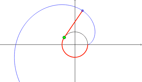
Involutes
Some curves are generated from others. An involute (also called evolvent) of a curve is the locus of the tip (or any other point) on a piece of taut string as the string is either unwrapped from or wrapped around the curve. Involutes were first studied by Huygens in 1673, particularly those of a cycloid, as part of his study on isochronous pendula. There are infinitely many involutes to a given curve, depending on the point where the tip of the string detaches from it, and also depending on the direction of the wrapping/unwrapping. In the figure below, an involute to a given circle is represented in blue color. Any other involute is obtained by rotation/reflection about a line through the origin.
Let us derive the equation of the involute of a general regular curve on the plane given parametrically:
,
where regularity means (if we think of the parameter as time, the point never stops during its motion). We can easily parametrize the involute using the same parameter . Namely, call the coordinates of the point of the involute on the tangent to at and let the length of the detached portion of the string (that is, the arc length measured from the point of detachment, also called natural parameter in Differential Geometry). In the figure below, we assume that the base curve is positively oriented, so the increase of the parameter corresponds to a counterclockwise motion along the curve. The values and represented correspond to . The string is also being unwrapped counterclockwise.
We have
,
where is the angle formed by the tangent at with the -axis.
On the other hand, from the differential triangle we see that
.
In terms of derivatives, we conclude
.
In the generał case, is obtained via integration from a given point
.
For a circle of unit radius, parametrized as , clearly if we choose the point as the starting point. An appplication of the general formula gives
Huygens also proved that the locus of the centers of curvature of any involute is the original curve, called the evolute. Huygens and his contemporaries defined the center of curvature as the “point of intersection of two infinitesimally close normals”. Nowadays we would say: ” the center of curvature is the center of the osculating circle”. This conceptual shift clearly shows the transition from a more dynamic to a more static point of view which runs in parallel with the abandonment of infinitesimals.
For algebraic curves, the osculating circle can be found by purely algebraic methods. Indeed, the osculating circle is the unique circle having order of tangency at least two with the curve at the given point. That was the method employed by Descartes. As Johann Bernoulli pointed out, this procedure breaks down for transcendental curves and has to be replaced by a more flexible method based on infinitesimal calculus.
I reproduce below Bernoulli’s derivation of a formula for the radius of the osculating circle (radius of curvature) as a function of and . It is representative of the Leibnizian calculus of infinitesimals. Remarkably, the result involves second differentials.
Let be a portion of a regular curve, with and being infinitesimally close points on it. Let the normals to the curve at and meet at . We choose the origin of coordinates at and pick the -axis so it intersects and at points and . We draw a vertical auxiliary line and a horizontal line through meeting at , and yet another vertical through meeting at . Finally, we draw , perpendicular to . Let the coordinates of and be (resp. ). Our goal is to compute the radius of curvature , in terms of , and their differentials and . Due to the local nature of , the final result will not depend on directly.
First, we observe that triangles , , are all similar (strictly or up to negligible infinitesimals) to the differential triangle . From the similarity of and we get
Writing and solving for ,
.
Using the triangle similarities mentioned above,
;
;
.
Putting all together,
.
Taking into account that our figure assumes (otherwise the point would be located above the curve and a few signs in the computations would change), and dividing throughout by we obtain the familiar formula
.
At points where , the osculating circle degenerates into a line and .
If the original curve is given in parametric form, ceases to be an independent variable and one has to modify the computation of above. Since one has
,
leading to the formula
,
where now derivatives are taken with respect to the parameter .
Compared with a modern derivation, the one above may rightfully seem a bit clumsy and lacking a systematic approach. It is more of an art; the art of recognizing quantities that can be disregarded in the pre-limit situation. However, apart from that, it is impressive how little is actually needed to get the formula. Just similarity of triangles!
Once we have a formula for the radius of curvature, deriving the equation of the evolute of a generic curve is straightforward. We obtain the point on the evolute by shifting the point in the direction of the normal by the amount .That is,
.
The formulas obtained allow to easily prove Huygens’ claim: a given curve is the evolute of any of its involutes. As a consequence, the evolute is the envelope of the family of normals of any of its involutes.
Involutes have cusps at the point where the string detaches from the curve. Evolutes have cusps at points corresponding to maximum/minimum curvature.
Some examples of involute/evolute pairs are: tractrix/catenoid, parabola/semicubic parabola, ellipse/(stretched) astroid, logarithmic spiral/(another) logarithmic spiral, &c.
In simple instances, tangency can be easily characterized. For example, a straight line is tangent to a circle precisely when they share a unique point. More generally, a curve which is the smooth boundary of a convex set has a unique tangent at each point, which can be characterized as the supporting line of the convex set.
But in more general cases such description is inadequate. For example, how do we characterize the tangent to the graph of a polynomial like at the point ? The epigraph is not convex, so the description as a supporting line is not available. Also, it clearly intersects the graph at some other point. Even worse, at the point the tangent actually crosses the graph, so the latter is not contained in either one of the two half-planes defined by the tangent, even locally. For polynomials, an algebraic definition of tangency in terms of the multiplicity of the point of tangency as a root to a polynomial equation is available, but in more general situations an analytic description is needed.
Finding tangents, along with finding areas, is one of the geometric problems that gave impetus to the use of infinitesimals and the eventual creation of Calculus. Predecessors of Newton and Leibniz, notably Fermat and Descartes, devised methods for finding tangents. For example, according to Fermat’s method, to find the tangent to the graph below at , he would choose a point on the graph, very close to , and would argue that the triangles and were “almost” similar. He then wrote an “adequality” (approximate proportion)
or, calling (the subtangent)
.
This, in turn, can be written as
.
Expanding and simplifying the left hand side and setting (a predecessor of “finding the derivative”) gives , being the slope of the tangent. When is a polynomial function of , this program can be easily carried out.
These ideas were further refined by Roverbal, Wallis, Barrow, Newton and Leibniz. The latter defined the tangent as the line through a pair of infinitely close points on the curve.
The modern analytic characterization is the following: the tangent line at a point of a curve has to be such that, as we move along the tangent towards the point of intersection with the curve, the distance to the graph in any “transversal” direction decreases to zero faster than the distance “along” the tangent to the point of intersection. That is, the curve is “transversally” closer to the tangent near the given point. In a sense, the neglect of the transversal separation between the triangles and is the key to Fermat’s construction. The following figure clarifies the situation further.
The line is tangent to the graph at if
when is infinitesimal. The transversal direction chosen is irrelevant. Had we chosen the direction in the above figure, we would still have , since as approaches , the curve and the tangent become “parallel” and the ratio stabilizes to some positive constant.
Notice that, for a non-tangent, transversal line through , the ratio is not infinitesimal, but rather stabilizes to a positive value depending on the final non-zero angle between the curve and the chosen non-tangent line.
It follows from our definition that the tangent is unique (if there is one). It is also worth noting that the concept of tangency belongs to Euclidean, as well as to affine geometries: tangency does not break down under rigid motions, translations and more general affine transformations (shear, dilations, etc.)
It is natural to quantify the “amount” of tangency by the order of the infinitesimal with respect to . Namely, we will say that the order of tangency is if
So, in particular, the order of tangency is zero if the line is transversal to the curve, it is one if is a quadratic infinitesimal, etc. The order of tangency may not be an integer.
Tangents and differentiability
The existence of the tangent to the curve at a point is intimately related to the existence of the first differential . To see why, we start by noticing that if the curve has a non-vertical tangent at (see figure below), the vertical distance between the graph and the tangent is also infinitesimal with respect to , because and are proportional, . Therefore
when is infinitesimal. But , where is the abscissa of the moving point .
If we assume that the straight line is tangent at , we should have
or
.
But this is precisely our definition of differentiable function at , with . Therefore, the existence of a tangent with slope implies differentiability with . The value of the derivative is the slope of the tangent.
If the order of tangency is , that is if
,
it follows from the definition that for .
As an example, let’s examine the order of tangency between a circle and its tangent at some point. For simplicity, consider the circle
with unit radius, center and tangent to the -axis at the origin , see the figure below.
We have , . Therefore,
as . Hence . Actually, is an infinitesimal of the second order with respect to . Indeed,
as . Thus and the order of tangency is .
The value of the limit would be different for circles of different radii. Indeed, if our circle was , since the numerator and denominator in scale differently, the limit would be .
The usual (linear) angle between a circle and its tangent at one point is zero. But our previous analysis allows to quantify the separation between the circle and the tangent using an infinitesimal quadratic scale. Observe that when is close to zero, is very large, whereas when is very large and the circle is “very close” to its tangent, is close to zero.
Angles like the above, whose usual measure is zero but their extent can be quantified as before, have been known since antiquity.
Horn angles
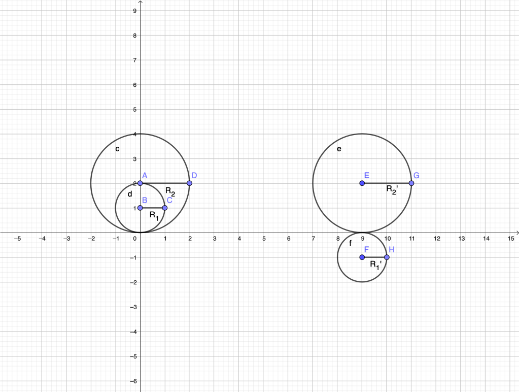
A horn angle is the angle formed between a circle and its tangent or, more generally, between two tangent circles at their point of tangency. Given two circles internally tangent, it is natural to define the measure of the horn angle between them as the difference of the angles they form with their common tangent. If they are externally tangent, we take the sum instead, as in the figure below.
Thus, in the first case, in the second. The factor is common and omitted for simplicity. For a circle of radius , the quantity is called its (scalar) curvature. The measure of a horn angle between two tangent circles is the difference/sum of their curvatures.
Horn angles are mentioned by Euclid in Book III (Prop. 16) of the “Elements”, and were known to Archimedes and Eudoxus. Euclid states that a horn angle is “smaller than any acute angle”. That property made horn angles problematic to Ancient Greek mathematicians, since they always assumed that any two “homogeneous” magnitudes (lengths, angles, areas, ..) were comparable, in the sense that anthyphairesis (as we would say today, the Euclidean algorithm) could be applied to them. At the end of the process, commensurable magnitudes could be assigned numbers with respect to some unit. Incommensurable magnitudes could not, but the situation could be handled by means of Eudoxus’ theory of proportions, a predecessor of Dedekind’s theory of real numbers. But the notion of a non-zero angle smaller than any acute angle was out of grasp. In modern terminology, we would say that the Archimedean property of segments, angles, areas was a basic assumption in Greek geometry.
We have been able to define a measure for horn angles using the concept of order of infinitesimals. However, to restore the Greeks’ assumption on the possibility to compare (albeit “in the limit”) any pair of angles, actual infinitesimal angles of different orders need to be included in the picture. This is the content of non-Archimedean Geometry, based on the construction of non-Archimedean fields (surreal, hyperreal numbers) in Nonstandard Analysis. The development of these ideas is a very interesting chapter of Analysis, well deserving a separate post, or even a separate thread.


![\left\{\begin{array}{l}\displaystyle{ \frac{dx}{dt}=f(t,x)} ;\\[10pt] x(t_0)=x_0 \end{array}\right.\qquad\qquad\qquad \textrm{(IVP)}](https://s0.wp.com/latex.php?latex=%5Cleft%5C%7B%5Cbegin%7Barray%7D%7Bl%7D%5Cdisplaystyle%7B+%5Cfrac%7Bdx%7D%7Bdt%7D%3Df%28t%2Cx%29%7D+%3B%5C%5C%5B10pt%5D+x%28t_0%29%3Dx_0+%5Cend%7Barray%7D%5Cright.%5Cqquad%5Cqquad%5Cqquad+%5Ctextrm%7B%28IVP%29%7D&bg=ffffff&fg=444444&s=0&c=20201002)


![[t,t_1]](https://s0.wp.com/latex.php?latex=%5Bt%2Ct_1%5D&bg=ffffff&fg=444444&s=0&c=20201002)


![\left\{\begin{array}{l}\displaystyle{ \frac{dy}{dt}=Ly} ;\\[10pt] y(t_1)=x_1 \end{array}\right.](https://s0.wp.com/latex.php?latex=%5Cleft%5C%7B%5Cbegin%7Barray%7D%7Bl%7D%5Cdisplaystyle%7B+%5Cfrac%7Bdy%7D%7Bdt%7D%3DLy%7D+%3B%5C%5C%5B10pt%5D+y%28t_1%29%3Dx_1+%5Cend%7Barray%7D%5Cright.&bg=ffffff&fg=444444&s=0&c=20201002)


![\left\{\begin{array}{l}\displaystyle{ \frac{dx}{dt}=x^{2/3}} ;\\[10pt] x(0)=0 \end{array}\right.](https://s0.wp.com/latex.php?latex=%5Cleft%5C%7B%5Cbegin%7Barray%7D%7Bl%7D%5Cdisplaystyle%7B+%5Cfrac%7Bdx%7D%7Bdt%7D%3Dx%5E%7B2%2F3%7D%7D+%3B%5C%5C%5B10pt%5D+x%280%29%3D0+%5Cend%7Barray%7D%5Cright.&bg=ffffff&fg=444444&s=0&c=20201002)


![\left\{\begin{array}{l}\displaystyle{ \frac{d\bar x}{ds}=g(s,\bar x):=f(s+t_0, \bar x+x_1(s+t_0))-f(s+t_0, x_1(s+t_0))} ;\\[10pt] \bar x(0)=0 \end{array}\right.](https://s0.wp.com/latex.php?latex=%5Cleft%5C%7B%5Cbegin%7Barray%7D%7Bl%7D%5Cdisplaystyle%7B+%5Cfrac%7Bd%5Cbar+x%7D%7Bds%7D%3Dg%28s%2C%5Cbar+x%29%3A%3Df%28s%2Bt_0%2C+%5Cbar+x%2Bx_1%28s%2Bt_0%29%29-f%28s%2Bt_0%2C++x_1%28s%2Bt_0%29%29%7D+%3B%5C%5C%5B10pt%5D+%5Cbar+x%280%29%3D0+%5Cend%7Barray%7D%5Cright.&bg=ffffff&fg=444444&s=0&c=20201002)


![\alpha\in (0,2]](https://s0.wp.com/latex.php?latex=%5Calpha%5Cin+%280%2C2%5D&bg=ffffff&fg=444444&s=0&c=20201002)


![\left\{\begin{array}{l}\displaystyle{ \frac{dx}{dt}=x^2} ;\\[10pt] x(t_0)=x_0>0 \end{array}\right.](https://s0.wp.com/latex.php?latex=%5Cleft%5C%7B%5Cbegin%7Barray%7D%7Bl%7D%5Cdisplaystyle%7B+%5Cfrac%7Bdx%7D%7Bdt%7D%3Dx%5E2%7D+%3B%5C%5C%5B10pt%5D+x%28t_0%29%3Dx_0%3E0+%5Cend%7Barray%7D%5Cright.&bg=ffffff&fg=444444&s=0&c=20201002)


![\left\{\begin{array}{l}\displaystyle{ \frac{dx}{dt}=\Psi(x)} \\[10pt] x(t_0)=x_0 \end{array}\right.](https://s0.wp.com/latex.php?latex=%5Cleft%5C%7B%5Cbegin%7Barray%7D%7Bl%7D%5Cdisplaystyle%7B+%5Cfrac%7Bdx%7D%7Bdt%7D%3D%5CPsi%28x%29%7D+%5C%5C%5B10pt%5D+x%28t_0%29%3Dx_0+%5Cend%7Barray%7D%5Cright.&bg=ffffff&fg=444444&s=0&c=20201002)


 . In other words, it is the locus of points equidistant from the focus and the directrix. A two line computation gives the equation
 and directrix
  . In a similar fashion the equations for the other conics can be obtained and used to derive further properties. Conic sections correspond to quadratic equations in two variables, a fact first established by Wallis in 1655.
 etc. which can be integrated in quadratures in some cases.
  at a generic point of the sought after curve was (and still is) a valuable tool in the derivation of the differential relations. Let’s look into some examples.
 – plane satisfying the following property: the area of the triangle defined by the tangent, the ordinate and the subtangent is a positive constant
  .
. , its ordinate by
  and the subtangent be
  (figure below).
 is tangent to the curve, the triangle
  is similar to the differential triangle at


 ,
, . As we move along one of these hyperbolas, the distance to the
  -axis is inversely proportional to the size of the subtangent.
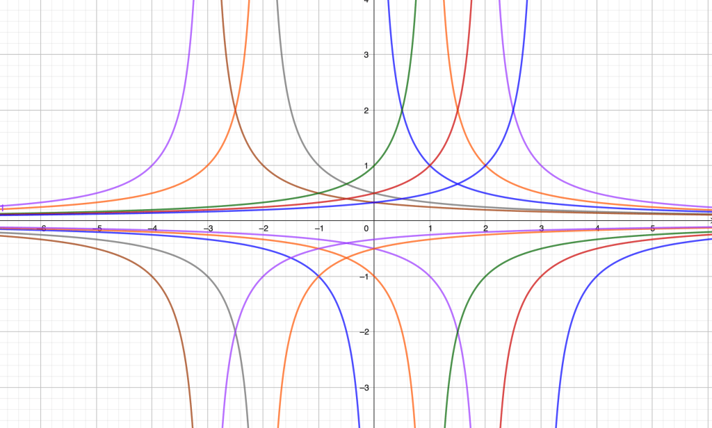
 -axis containing the point where the object is initially located. Let
  be the initial distance from the object to the
  . We look at this problem from a strictly geometric point of view, assuming that the object is a mass point that reacts instantly to the pulling force, aligning its motion with the force at all times. In other words, the goal is to find a curve whose segment of tangent between the point of tangency and the
  is the point of intersection between the tangent at
  is the foot of the perpendicular from
  is the abscissa). Here,
  .
.
 .
. 
 .
. then reads
 ,
, ) adding the condition
  gives
gives
 on the plane given parametrically:
 ,
, (if we think of the parameter
  the coordinates of the point of the involute on the tangent to
  and let
  the length of the detached portion of the string (that is, the arc length measured from the point of detachment, also called natural parameter in Differential Geometry). In the figure below, we assume that the base curve is positively oriented, so the increase of the parameter
  and
and  represented correspond to
  . The string is also being unwrapped counterclockwise.
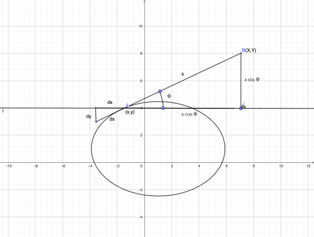
 ,
, is the angle formed by the tangent at
  .
.  .
.  .
. , clearly
  if we choose the point
  as the starting point. An appplication of the general formula gives
 and
and  . It is representative of the Leibnizian calculus of infinitesimals. Remarkably, the result involves second differentials.
 be a portion of a regular curve, with
  and
and  being infinitesimally close points on it. Let the normals to the curve at
  . We choose the origin of coordinates at
  and pick the
  and
and  at points
  and
and  . We draw a vertical auxiliary line
  and a horizontal line through
  , and yet another vertical through
  at
at  . Finally, we draw
  , perpendicular to
  (resp.
  ). Our goal is to compute the radius of curvature
  , in terms of
  ,
,  and their differentials
  and
and  . Due to the local nature of
  directly.
 ,
,  ,
,  are all similar (strictly or up to negligible infinitesimals) to the differential triangle
  . From the similarity of
  and
and  we get
 and solving for
  .
. ;
; ;
; .
. .
. (otherwise the point
  we obtain the familiar formula
 .
. , the osculating circle degenerates into a line and
  .
. above. Since
  one has
 ,
, ,
, on the evolute by shifting the point
  by the amount
  .That is,
  .
. at the point
  ? The epigraph is not convex, so the description as a supporting line is not available. Also, it clearly intersects the graph at some other point. Even worse, at the point
  the tangent actually crosses the graph, so the latter is not contained in either one of the two half-planes defined by the tangent, even locally. For polynomials, an algebraic definition of tangency in terms of the multiplicity of the point of tangency as a root to a polynomial equation is available, but in more general situations an analytic description is needed.
 , he would choose a point
  on the graph, very close to
  and
and  were “almost” similar. He then wrote an “adequality” (approximate proportion)

 (the subtangent)
 .
. .
. (a predecessor of “finding the derivative”) gives
  ,
,  being the slope of the tangent. When
  is a polynomial function of
  and
and  is the key to Fermat’s construction. The following figure clarifies the situation further.
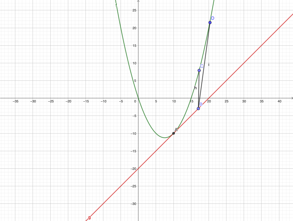

 is infinitesimal. The transversal direction chosen is irrelevant. Had we chosen the direction
  , since as
  stabilizes to some positive constant.
  is not infinitesimal, but rather stabilizes to a positive value depending on the final non-zero angle between the curve and the chosen non-tangent line.
  with respect to
  if
if 
 at a point
  is intimately related to the existence of the first differential
  . To see why, we start by noticing that if the curve
  , because
  . Therefore
 , where
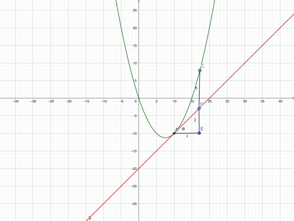
 is tangent at
 ![|BC|=y(x)-[y_0+m(x-x_0)]=o(|x-x_0|)](https://s0.wp.com/latex.php?latex=%7CBC%7C%3Dy%28x%29-%5By_0%2Bm%28x-x_0%29%5D%3Do%28%7Cx-x_0%7C%29&bg=ffffff&fg=444444&s=0&c=20201002)
 .
. , with
  . Therefore, the existence of a tangent with slope
  . The value of the derivative is the slope of the tangent.
  , that is if
 ,
, for
for  .
. 
 and tangent to the
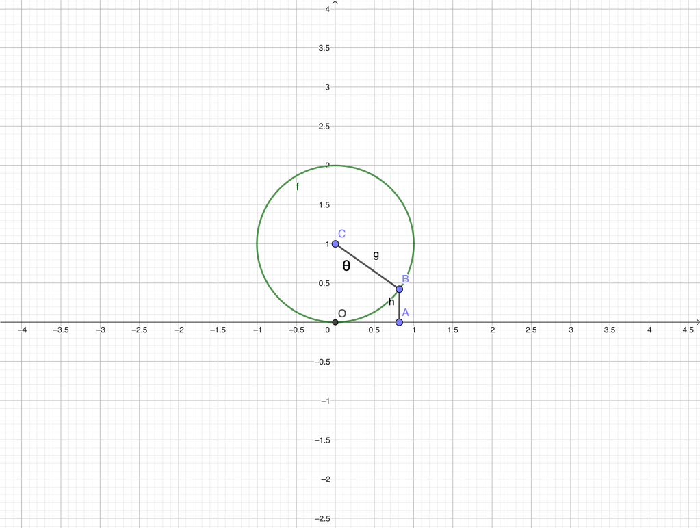
 ,
,  . Therefore,
 . Hence
  . Actually,
  . Indeed,
 and the order of tangency is
  .
. would be different for circles of different radii. Indeed, if our circle was
  , since the numerator and denominator in
  .
. 
 in the first case,
  in the second. The factor
  is common and omitted for simplicity. For a circle of radius
  is called its (scalar) curvature. The measure of a horn angle between two tangent circles is the difference/sum of their curvatures.