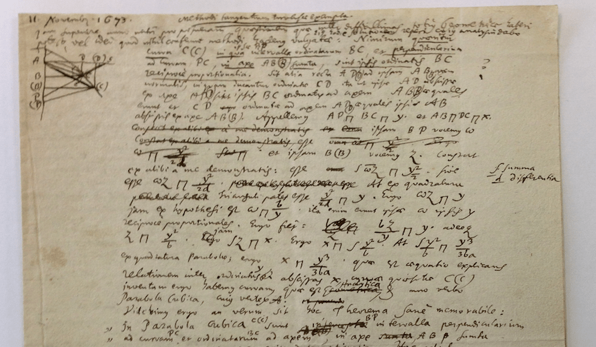
In pre-epsilontic times, mathematicians understood definite integrals as continuous sums of infinitesimals (in the above image, a page from Leibniz where he introduces the signs 


Let us recall the definitions for the sake of completeness. For a real function of a real variable 


Both derivatives and integrals are limits. The derivative of 

whenever the latter is finite. In the case of the definite integral over ![[a,b]](https://s0.wp.com/latex.php?latex=%5Ba%2Cb%5D&bg=ffffff&fg=444444&s=0&c=20201002)


![\xi_i\in [x_{i-1},x_i]](https://s0.wp.com/latex.php?latex=%5Cxi_i%5Cin+%5Bx_%7Bi-1%7D%2Cx_i%5D&bg=ffffff&fg=444444&s=0&c=20201002)

If the above sums have a finite limit 


I am not concerned here with the alternative constructions of the continuum and the non-standard approach. My main concern is the teaching of (standard) Calculus. It is my belief that the main difficulties encountered by students when faced with the above definitions are philosophical/psychological in nature, as they feel a disconnection with good old Algebra and finite procedures. In order to fill the gap, I believe that the language of infinitesimals is to be preferred, specially in introductory courses. As I pointed out elsewhere, this is the language used by most users of Calculus, including Physicists and Engineers. Just like derivatives are quotients of infinitesimals, integrals are sums of infinitesimals, thus revealing a common theme. In other words, I believe that Calculus should be presented as an algebra of infinitesimals.
The main objection to this approach is the fact that infinitesimals cannot be properly defined in the realm of standard Calculus, based on the standard real line. I believe however that the pedagogical advantages stemming from its more intuitive character and its agreement with the historical evolution of the subject is worth the lack of rigor on a first acquaintance with the subject.
Let’s consider the different types of sums used in Calculus.
Adding two numbers is an operation everyone is familiar with. The (inductive) extension to a finite amount of addends is trivial, thanks to associativity. Here we are in the realm of Algebra.
Things become trickier when we intend to add infinitely many numbers. We already encounter this situation In Zeno’s paradoxes: In order to travel a certain distance, say 

Standard modern mathematics, however, has embraced the idea of the continuum through the concept of real number, originated with Simon Stevin and his decimal representations. Thanks to a hypostatic abstraction, now we declare numbers (real numbers) a certain property of sequences of rational numbers. In simpler terms, we adjoin to the number system all potential “limits”. Such construction would have abhorred Eudoxus and Euclid, but Cantor and Dedekind, along with most current mathematicians, were perfectly comfortable with it. In order to circumvent Zeno’s paradox, we start by defining the concept of infinite sum. The simplest choice, as is well known, is to consider “partial sums”

which in this case can be easily computed in closed form, 


Several comments are in order. 


which is the “irrational” number 
A necessary condition for the series 


As an example of the first mechanism, any series of geometrically decreasing terms like the one above is convergent. Also, any series whose terms behave asymptotically as those of a convergent geometric series is convergent (this is called the ratio test). A relevant example of cancellation is given by Leibniz’s series 

Summing up, for a sum over a discrete set of indices to be finite, the terms have to become small in a way that balances the number of addends, stabilizing the partial sums towards a finite limit.
Definite integrals showcase the next level of summation. In Riemann’s construction with uniform partitions, generic terms of the Riemann sums are of the order of 


over the set of indices ![I=[a,b]](https://s0.wp.com/latex.php?latex=I%3D%5Ba%2Cb%5D&bg=ffffff&fg=444444&s=0&c=20201002)

When a Physicist needs to find the total mass of a non-homogeneous bar with density 


Physics and Engineering books contain plenty of such formulas to compute extensive magnitudes. Yet the way Calculus is currently taught is at odds with the above line of thought. A colleague engineer once told me “I had to relearn Calculus. The version mathematicians taught me was useless”.
The balance between the cardinality of the set of indices and the size of the terms is critical. For instance, if we consider “Riemann sums” of either form

the corresponding limits are trivial,

for “reasonable” (say, continuous on 

We can further consider sums over a doubly continuous set of indices ![I=[a,b]\times[c,d]](https://s0.wp.com/latex.php?latex=I%3D%5Ba%2Cb%5D%5Ctimes%5Bc%2Cd%5D&bg=ffffff&fg=444444&s=0&c=20201002)
![\displaystyle{\iint\limits_{[a,b]\times[c,d]} f(x,y)\, dxdy}](https://s0.wp.com/latex.php?latex=%5Cdisplaystyle%7B%5Ciint%5Climits_%7B%5Ba%2Cb%5D%5Ctimes%5Bc%2Cd%5D%7D+f%28x%2Cy%29%5C%2C+dxdy%7D&bg=ffffff&fg=444444&s=0&c=20201002)
where the addends are quadratic infinitesimals 

![\displaystyle{\iint\limits_{[a,b]\times[c,d]}f(x,y)\,dx^2dy=0};\qquad\displaystyle{\iiint\limits_{[a,b]\times [c,d]\times [e,f]}f(x,y,z)\,dxdz=\infty}](https://s0.wp.com/latex.php?latex=%5Cdisplaystyle%7B%5Ciint%5Climits_%7B%5Ba%2Cb%5D%5Ctimes%5Bc%2Cd%5D%7Df%28x%2Cy%29%5C%2Cdx%5E2dy%3D0%7D%3B%5Cqquad%5Cdisplaystyle%7B%5Ciiint%5Climits_%7B%5Ba%2Cb%5D%5Ctimes+%5Bc%2Cd%5D%5Ctimes+%5Be%2Cf%5D%7Df%28x%2Cy%2Cz%29%5C%2Cdxdz%3D%5Cinfty%7D&bg=ffffff&fg=444444&s=0&c=20201002)
etc.
I believe formulas like 

References:
[1] “Ten misconceptions from the history of Analysis and their debunking”, P. Blaszczyk, M.G. Katz and D. Sherry, https://arxiv.org/pdf/1202.4153.pdf
[2] “Elements of the history of Mathematics”, N. Bourbaki, Springer Science & Business Media, 1998.
