September | 2023 | Math Bites

Sets of points satisfying certain geometric condition are ubiquitous in Mathematics. The simplest examples are straight lines, circles and more general conics. Thus a straight line can be defined as the set of points equidistant from two given points, a circle as the set of points whose distance to a fixed point (center) is constant and a conic as the set of points such that the ratio of the distances to a given point (focus) and a given line (directrix) is constant. The type of conic depends on whether the ratio (called eccentricity) is less, equal or greater than one.

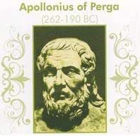
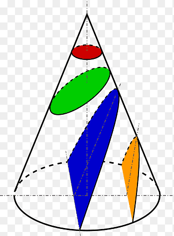
Straight lines and circles were intensively studied since antiquity. They were the favorite objects of Greek geometers, and their properties are thoroughly investigated in Euclid’s Elements. In his fundamental treatise “Conics”, Apollonius of Perga, known as the “Great Geometer”, went further, tackling a systematic study of conics, establishing their focal properties, as well as those of chords and tangents, “conjugate” diameters, asymptotes, etc. It is believed that he heavily drew from previous work by Euclid as well as from Menaechmus, who is generally considered the discoverer of conic sections.

Greeks did not stop there. For the purpose of solving construction problems not amenable to the straightedge and the compass, they introduced more sophisticated loci like conchoids and cissoids, and “kinematic” curves like the quadratrix or the Archimedean spiral.

When the method of coordinates was introduced by Fermat and Decartes in the XVII century, the sophisticated auxiliary constructions typical of synthetic geometry were replaced by more straightforward and systematic algebraic methods. The equations of the above mentioned curves were obtained right away by expressing their defining properties in the language of Algebra. For instance, a parabola is a conic with eccentricity $e=1$ . In other words, it is the locus of points equidistant from the focus and the directrix. A two line computation gives the equation

$y^2=2px$

for a parabola with focus at $F(p,0)$ and directrix $x=-p$ . In a similar fashion the equations for the other conics can be obtained and used to derive further properties. Conic sections correspond to quadratic equations in two variables, a fact first established by Wallis in 1655.

Yet another locus, also considered by the Greeks, is that of points such that the ratio of their distances to two given points is constant. Using coordinates, one easily arrives at the equation of a circle (or a line if the ratio is equal to one). These are the so called Apollonian circles. They appear in applications, for instance as the zero-potential line for a system of two point charges in Electrostatics.

In the previous examples, the property defining the curve could be directly translated into a finite algebraic relation between the coordinates. With the birth of Calculus other classes of curves started to draw the attention of scholars, namely those whose defining property was more “local” in nature, in the sense that it involved the direction or some other feature of the curve at each point. In those cases, the defining property is not a finite, but rather a differential equation, relating $x, y, dx, dy, d^2y$ etc. which can be integrated in quadratures in some cases.

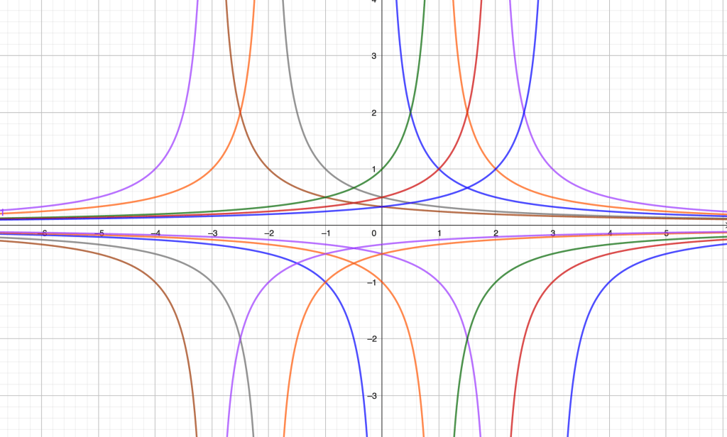
The consideration of the “differential triangle” with sides $dx,dy$ at a generic point of the sought after curve was (and still is) a valuable tool in the derivation of the differential relations. Let’s look into some examples.

A family of equilateral hyperbolas

Consider the locus of points on the $XY$ – plane satisfying the following property: the area of the triangle defined by the tangent, the ordinate and the subtangent is a positive constant $a^2$ .

Let the generic point be $P(x,y)$ , its ordinate by $PQ$ and the subtangent be $QR$ (figure below).

Since $PR$ is tangent to the curve, the triangle $\Delta PQR$ is similar to the differential triangle at $P$ . Therefore,

$\displaystyle{\frac{dy}{dx}=\frac{PQ}{QR}=\frac{\pm y}{QR}}$

and, consequently

$\displaystyle{QR=\pm y\frac{dx}{dy}}$

The given condition then reads

$\displaystyle{\pm y^2 dx=2a^2dy}$

$\displaystyle{\frac{dy}{y^2}\pm\frac{dx}{2a^2}=0}$

The expression on the left is a total differential,

$\displaystyle{d\left(-\frac 1{y}\pm \frac{x}{2a^2}\right)=0}$

giving a general solution of the form

$\displaystyle{y=\frac{2a^2}{C\pm x}}$ ,

which is a family of equilateral hyperbolas with common asymptote $y=0$ . As we move along one of these hyperbolas, the distance to the $Y$ -axis is inversely proportional to the size of the subtangent.

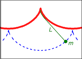
The tractrix

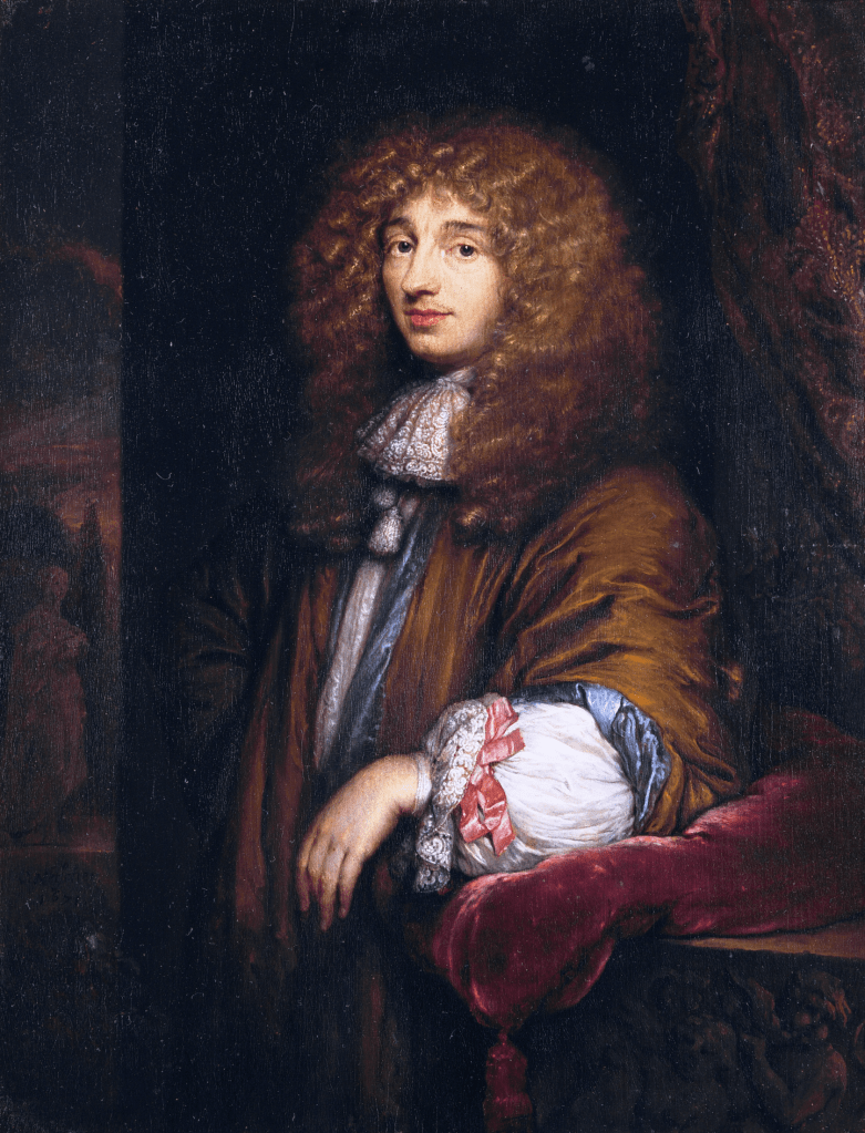
The following problem was proposed by Claude Perrault in1670, solved in 1692 by Huygens and subsequently solved by Leibniz, Johann Bernoulli and others.

“What is the path of an object dragged along a horizontal plane by a string of constant length when the end of the string not joined to the object moves along a straight line in the plane?”

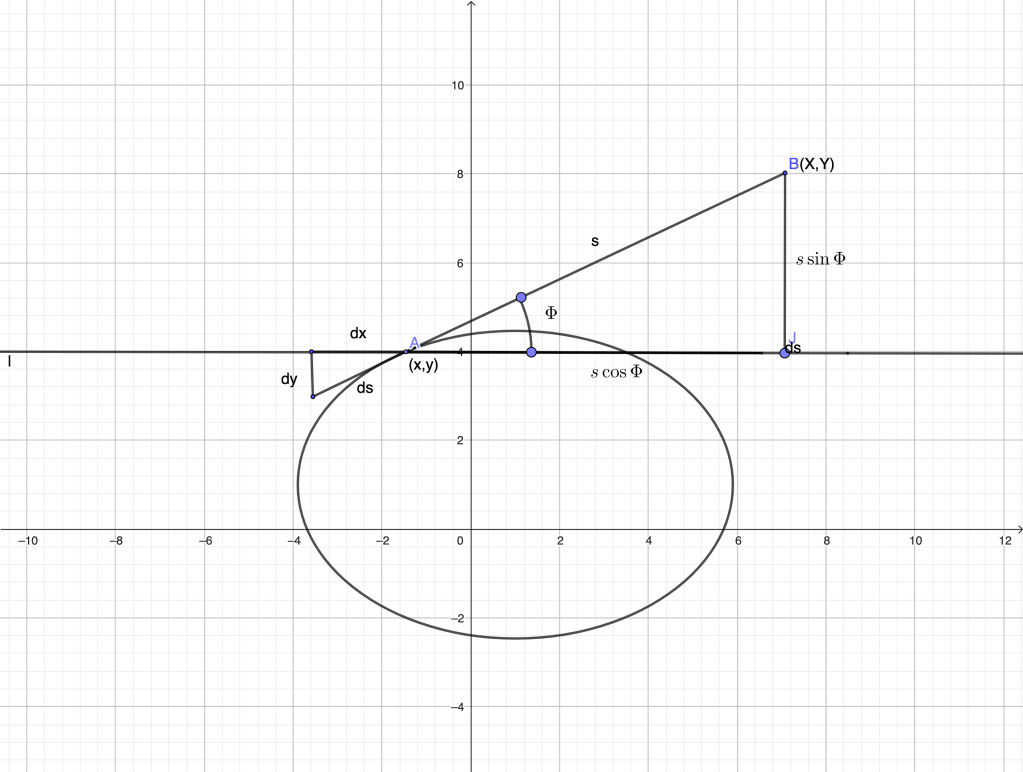
Obviously, if the object is initially on the line of the force, the path is just a line. Assume it is not. For simplicity, choose the $Y$ -axis in the direction of the force and the $X$ -axis containing the point where the object is initially located. Let $a$ be the initial distance from the object to the $Y$ -axis (equal to the length of the string) so the initial position is $(a,0)$ . We look at this problem from a strictly geometric point of view, assuming that the object is a mass point that reacts instantly to the pulling force, aligning its motion with the force at all times. In other words, the goal is to find a curve whose segment of tangent between the point of tangency and the $Y$ -axis has constant length, equal to $a$ .

In the figure, $P$ is a generic point on the curve, $Q$ is the point of intersection between the tangent at $P$ and the vertical axis and $R$ is the foot of the perpendicular from $P$ to the axis (so $RP$ is the abscissa). Here, $a=5$ .

The condition to be satisfied is $|PQ|=a$ .

The triangle $\Delta PQR$ and the differential triangle are similar, as before. Therefore,

$\displaystyle{-\frac{dy}{dx}=\frac {|QR|}{|RP|}}$

thus implying

$\displaystyle{|QR|=-|RP|\frac{dy}{dx}=-x\frac{dy}{dx}}$ .

The condition $|QP|^2=|RP|^2+|QR|^2$ then reads

$\displaystyle{x^2+x^2\left(\frac{dy}{dx}\right)^2=a^2},$

equivalent to two differential equations,

$\displaystyle{\frac{dy}{dx}=\pm\frac{\sqrt{a^2-x^2}}{x}}$ ,

Direct integration (say, by setting $x=a\cos\theta$ ) adding the condition $y(a)=0$ gives

$\displaystyle{y=\pm\left(a\ln \frac{a+\sqrt{a^2-x^2}}{x} -\sqrt{a^2-x^2}\right)}$

corresponding to an upper branch with negative slope (puller moving up) and a lower branch with positive slope (puller moving down). The branches meet at the initial point $(a,0)$ , which is a cusp. The vertical axis is an asymptote.

As it happens, if a tractrix is rotated about the asymptote, the obtained surface is a pseudosphere, whose Gaussian curvature is a negative constant (just like the Gaussian curvature on a sphere is a positive constant). The local geometry on a pseudosphere is hyperbolic, as shown by E. Beltrami.

Involutes

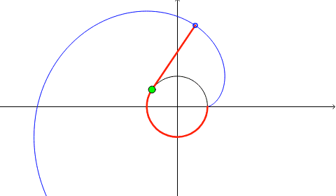
Some curves are generated from others. An involute (also called evolvent) of a curve is the locus of the tip (or any other point) on a piece of taut string as the string is either unwrapped from or wrapped around the curve. Involutes were first studied by Huygens in 1673, particularly those of a cycloid, as part of his study on isochronous pendula. There are infinitely many involutes to a given curve, depending on the point where the tip of the string detaches from it, and also depending on the direction of the wrapping/unwrapping. In the figure below, an involute to a given circle is represented in blue color. Any other involute is obtained by rotation/reflection about a line through the origin.

Let us derive the equation of the involute of a general regular curve $\gamma$ on the plane given parametrically:

$\gamma: x=x(t);\quad\quad y=y(t)$ ,

where regularity means $x'(t)^2+y'(t)^2\neq 0$ (if we think of the parameter $t$ as time, the point never stops during its motion). We can easily parametrize the involute using the same parameter $t$ . Namely, call $(X(t), Y(t))$ the coordinates of the point of the involute on the tangent to $\gamma$ at $(x(t),y(t))$ and let $s$ the length of the detached portion of the string (that is, the arc length measured from the point of detachment, also called natural parameter in Differential Geometry). In the figure below, we assume that the base curve is positively oriented, so the increase of the parameter $t$ corresponds to a counterclockwise motion along the curve. The values $dx$ and $dy$ represented correspond to $dt>0$ . The string is also being unwrapped counterclockwise.

We have

$X(t)=x(t)+s\cos\phi;\qquad Y(t)=y(t)+s\sin\phi$ ,

where $\phi$ is the angle formed by the tangent at $(x(t),y(t))$ with the $X$ -axis.

On the other hand, from the differential triangle we see that

$\cos\phi=-dx/ds;\qquad \qquad \sin\phi=-dy/ds;\qquad ds=\sqrt{dx^2+dy^2}$ .

In terms of derivatives, we conclude

$\displaystyle{X(t)=x(t)-s\frac{x'(t)}{\sqrt{x'(t)^2+y'(t)^2}};\qquad Y(t)=y(t)-s\frac{y'(t)}{\sqrt{x'(t)^2+y'(t)^2}}}$ .

In the generał case, $s$ is obtained via integration from a given point

$\displaystyle{s=\int\limits_{t_0}^tds=\int\limits_{t_0}^t\sqrt{x'(t)^2+y'(t)^2}\,dt}$ .

For a circle of unit radius, parametrized as $x=\cos t,\, y=\sin t$ , clearly $s=t$ if we choose the point $(1,0)$ as the starting point. An appplication of the general formula gives

$\displaystyle{X(t)=\cos t + t\sin t;\qquad Y(t)=\sin t - t\cos t}.$

The involutes of a circle are used in the design of gear teeth, see https://www.marplesgears.com/2019/10/an-in-depth-look-at-involute-gear-tooth-profile-and-profile-shift/

Evolutes

Huygens also proved that the locus of the centers of curvature of any involute is the original curve, called the evolute. Huygens and his contemporaries defined the center of curvature as the “point of intersection of two infinitesimally close normals”. Nowadays we would say: ” the center of curvature is the center of the osculating circle”. This conceptual shift clearly shows the transition from a more dynamic to a more static point of view which runs in parallel with the abandonment of infinitesimals.

For algebraic curves, the osculating circle can be found by purely algebraic methods. Indeed, the osculating circle is the unique circle having order of tangency at least two with the curve at the given point. That was the method employed by Descartes. As Johann Bernoulli pointed out, this procedure breaks down for transcendental curves and has to be replaced by a more flexible method based on infinitesimal calculus.

I reproduce below Bernoulli’s derivation of a formula for the radius of the osculating circle (radius of curvature) as a function of $x,y,dx,dy$ and $d^2y$ . It is representative of the Leibnizian calculus of infinitesimals. Remarkably, the result involves second differentials.

Let $ABO$ be a portion of a regular curve, with $B$ and $O$ being infinitesimally close points on it. Let the normals to the curve at $B$ and $O$ meet at $D$ . We choose the origin of coordinates at $A$ and pick the $X$ -axis so it intersects $BD$ and $OD$ at points $H$ and $G$ . We draw a vertical auxiliary line $BE$ and a horizontal line through $B$ meeting $OD$ at $C$ , and yet another vertical through $O$ meeting $BC$ at $F$ . Finally, we draw $GL$ , perpendicular to $BD$ . Let the coordinates of $B$ and $O$ be $(x,y)$ (resp. $(x+dx, y+dy)$ ). Our goal is to compute the radius of curvature $R=BD$ , in terms of $x=AE$ , $y=EB$ and their differentials $dx=BF$ and $dy=OF$ . Due to the local nature of $R$ , the final result will not depend on $x,y$ directly.

First, we observe that triangles $\Delta OFC$ , $\Delta BEH$ , $\Delta GLH$ are all similar (strictly or up to negligible infinitesimals) to the differential triangle $\Delta BFO$ . From the similarity of $\Delta DHG$ and $\Delta DBC$ we get

$\displaystyle{\frac{BD}{HD}=\frac{BC}{HG}}$

Writing $HD=BD-BH$ and solving for $BD$ ,

$\displaystyle{BD=\frac{BC\dot BH}{BC-HG}}$ .

Using the triangle similarities mentioned above,

$\displaystyle{BC=BF+FC=BF+\frac{FO^2}{BF}=dx+\frac{dy^2}{dx}=\frac{dx^2+dy^2}{dx}}$ ;

$\displaystyle{BH=\sqrt{BE^2+EH^2}=\sqrt{BE^2+\left(\frac{BE\cdot FO}{BF}\right)^2}=\sqrt{y^2+\left(\frac{ydy}{dx}\right)^2}=\frac{y\sqrt{dx^2+dy^2}}{dx}}$ ;

$\displaystyle{HG=dAH=d(AE+EH)=d\left(x+\frac{ydy}{dx}\right)=dx+\frac{yd^2y+dy^2}{dx}}$ .

Putting all together,

$\displaystyle{R=BD=\frac{(dx^2+dy^2)^{3/2}}{-dxd^2y}}$ .

Taking into account that our figure assumes $d^2y<0$ (otherwise the point $D$ would be located above the curve and a few signs in the computations would change), and dividing throughout by $dx^3$ we obtain the familiar formula

$\displaystyle{R=\frac{\left(1+y'^2\right)^{3/2}}{|y''|}}$ .

At points where $y''=0$ , the osculating circle degenerates into a line and $R=\infty$ .

If the original curve is given in parametric form, $x$ ceases to be an independent variable and one has to modify the computation of $HG$ above. Since $d^2x\neq 0$ one has

$\displaystyle{d\left(x+\frac{ydy}{dx}\right)=dx+\frac{(yd^2y+dy^2)dx-ydyd^2x}{dx^2}}$ ,

leading to the formula

$R(t)=\displaystyle{\frac{\left(x'^2+y'^2\right)^{3/2}}{|y''x'-x''y'|}}$ ,

where now derivatives are taken with respect to the parameter $t$ .

Compared with a modern derivation, the one above may rightfully seem a bit clumsy and lacking a systematic approach. It is more of an art; the art of recognizing quantities that can be disregarded in the pre-limit situation. However, apart from that, it is impressive how little is actually needed to get the formula. Just similarity of triangles!

Once we have a formula for the radius of curvature, deriving the equation of the evolute of a generic curve is straightforward. We obtain the point $(X(t),Y(t))$ on the evolute by shifting the point $(x(t),y(t))$ in the direction of the normal $(-dy,dx)$ by the amount $R(t)$ .That is,

$\displaystyle{X(t)=x(t)-\frac{y'(t)R(t)}{\sqrt{x'(t)^2+y'(t)^2}}};\quad \displaystyle{Y(t)=y(t)+\frac{x'(t)R(t)}{\sqrt{x'(t)^2+y'(t)^2}}}$ .

The formulas obtained allow to easily prove Huygens’ claim: a given curve is the evolute of any of its involutes. As a consequence, the evolute is the envelope of the family of normals of any of its involutes.

Involutes have cusps at the point where the string detaches from the curve. Evolutes have cusps at points corresponding to maximum/minimum curvature.

Some examples of involute/evolute pairs are: tractrix/catenoid, parabola/semicubic parabola, ellipse/(stretched) astroid, logarithmic spiral/(another) logarithmic spiral, &c.

A series of videos showing several involute/evolute pairs and how they are generated can be found here https://kmr.dialectica.se/wp/research/math-rehab/learning-object-repository/geometry-2/metric-geometry/euclidean-geometry/geometry/plane-curves/evolutes/

Math Bites

by Guillermo Reyes, PhD

Month: September 2023

Geometric loci

A family of equilateral hyperbolas

The tractrix

Involutes

Evolutes