Before we move onto concrete examples, let us quickly review some basic differentiation rules. In order to differentiate equations of the form

we need to replace all the variables 


For example, if 


since 


To differentiate an equation involving a product, 

and, since 

Let us next find 


Now, we observe that

Hence, up to linear terms,

and therefore

where we have disregarded the quadratic term 


Successive applications of the product rule give the important power rule:

and, in general, 
What about irrational/transcendental functions? As for 

by just rearranging the power rule. Therefore, the power rule extends to rational powers.
Let’s move now to the fun part.
Reasoning with infinitesimals
Suppose we want to compute 


where the trigonometric identity for the difference of sines has been used, as well as the fact that 

In the figure below, the unit circle is represented, and we consider a generic angle 

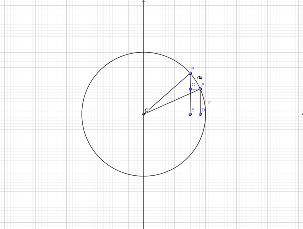
The corresponding change of 


From the perspective of rigor, the above argument is flawed, for many reasons. The “triangle” 


Admittedly, this type of argument relies on the ability to recognize which approximations will become exact in the limit. We believe this is a skill worth developing.
Here is another example mentioned in the beautiful book [1] and attributed there to Newton. Let us show that 


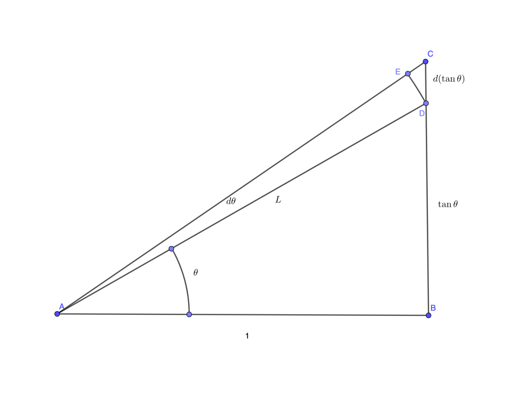
The triangles 

or

(because 


Solving problems using differentials
Let’s start with a simple optimization problem which is more elegantly solved using differentials.
Consider a sliding segment of length 

The standard approach to the problem is to express the area of the triangle as a function of some parameter (the horizontal projection of the segment, some angle, etc.) and find the value of the parameter that makes the derivative equal to zero. A more “symmetric” approach would be as follows. Let 


Differentiating both relations,

A necessary condition for 

For the above homogeneous linear system to have a non-trivial solution (so infinitesimal changes 


If we were to follow the approach based on derivatives, we could either express 

We would then find 
A similar example is presented in [2]. There, the classical problem of minimizing the length of a piece-wise straight path connecting two given points with a given line (so called Heron’s problem) is solved.

The given quantities (see Fig. above) are 


Differentiating all the equations gives

The condition of extremum is 


The determinant should be zero, that is 

and, consequently, 

Observe in particular that 
In both examples above, we solved a conditional optimization problem. A possible approach is to use the method of Lagrange multipliers. Thus in our case we are trying to. minimize

under the constraint

The main advantage of that method is to keep the symmetry between the variables, at the expense of introducing a number of multipliers. On our next post, we will discuss how the method was introduced by Lagrange to deal with constraints in mechanical systems. Not surprisingly, infinitesimals were at the heart of his analysis, in the form of virtual displacements.
References:
[1] T. Needham, “Visual Complex Analysis”, Oxford University Press, 1999.
[2] T. Dray, Corinne A. Manogue, “Putting Differentials Back into Calculus”, The College Mathematics Journal 42 (2), 2010.
